![[OLD FALL 2018] 15-104 • Introduction to Computing for Creative Practice](https://courses.ideate.cmu.edu/15-104/f2018/wp-content/uploads/2020/08/stop-banner.png)
/*Kevin Riordan
Section C
kzr@andrew.cmu.edu
project_07*/
function setup() {
createCanvas(480,480);
}
//this function checks whether a point is close enough to the step value to be drawn
function latticeCloseEnough(xc, yc, c1X, c1Y, c2X, c2Y, step, bSquare) {
//define two variables that the function will return for the if case in draw
var smaller = false;
var bigger = false;
//checking four corners of the "rectangle" i have defined around the point xc, yc
for(var x = xc - step/2; x <= xc + step/2; x += step){
for(var y = yc - step/2; y <= yc + step/2; y += step){
//distance used to check
r1r2 = dist(x,y,c1X,c1Y) * dist(x,y,c2X,c2Y)
if (r1r2 <= bSquare) smaller = true;
else bigger = true;
}
}
return smaller & bigger;
}
//this is my curve function for cassiniOvals on mathworld
function cassiniOvals(c1X, c1Y, c2X, c2Y, colorStretch) {
//this step variable determines how defined the latticegrid is, higher numbers make it very defined but lag the program badly
var step = 8;
//formula for this curve is dist1 * dist 2 = b^2
var dist1 = dist(c1X, c1Y, mouseX, mouseY);
var dist2 = dist(c2X, c2Y, mouseX, mouseY);
var bSquare = dist1 * dist2;
//these drew intermediate points used to test code
//point(c1X,c1Y);point(c2X,c2Y);
//these variables determine how wide and how many curves are drawn around the center points for each oval function
var range = 3;
var scale = 0.2;
var start = 4;
//converts bsquare into an array
var bSquareArray = Array.apply(null, Array(range)).map(function (_, i) {return bSquare * scale * (i + start);});
//drawing the ovals by checking across each point on the canvas, as determined by the step variable
for (var y = 0; y <= height; y += step) {
for (var x = 0; x <= width; x += step) {
for (var pos = 0; pos < bSquareArray.length; pos ++) {
var posColor = map(pos,0,range - 1,0,255);
//changing the color for each size of oval in each cassiniOval
stroke((posColor + 50) * colorStretch,(posColor - 50) * colorStretch,posColor * colorStretch);
//calling the latticechecking function to see if a point should be drawn
if(latticeCloseEnough(x, y, c1X, c1Y, c2X, c2Y, step, bSquareArray[pos])){
point(x,y);
}
}
}
}
}
function draw() {
background(0);
strokeWeight(2.5);
//left center coordinates
var c1X = width / 2;
var c1Y = height / 2;
//started by having two variables c1x and c2x when testing one cassiniOval, but both centers ended up only depending on c1x
//var c2X = 7*width/8;
var c2Y = height / 2;
var amount = 4;
//drawing the cassiniOVals
for (var i = 1; i <= 2; i += (1 / amount)) {
//declaring variable to change the color for each complete cassiniOval function
var colorStretch = map(i,0,2,0.1,1);
cassiniOvals(c1X * i,c1Y,c1X * (2 - i),c2Y, colorStretch);
}
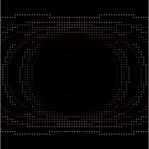
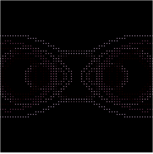
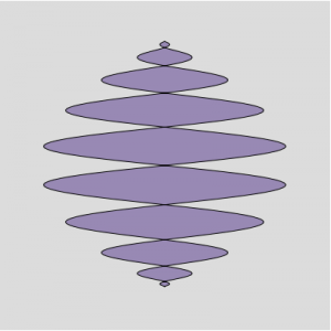
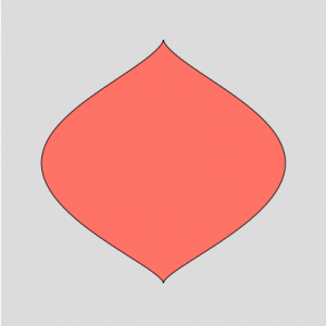
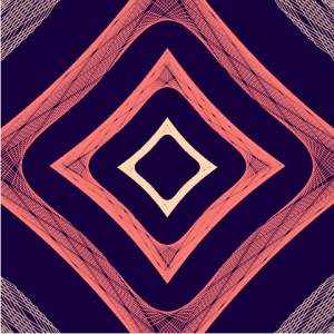
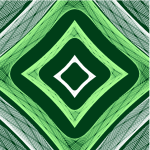
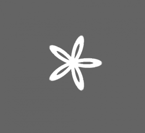
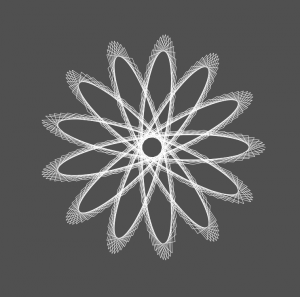
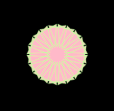
}This project was really cool to me. I used the Cassini Oval curve for this project from the MathWorld site. The main part of this project for me was creating a lattice checking function, so that the points did not get wider apart as the distances from the centers increased for larger increments. When I used a basic distance checking function, when the b-squared distance increased, the “bands” of points got thicker. I also used the .apply function I found online, which was hard for me to learn at first because I did not know about lambda expressions. Overall, this project really forced me to learn how to reorganize my code and the structure overall.
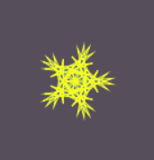
Below is a screenshot on the right of a standard overlapping Cassini ovals when distance is short, and another screenshot on the left when the mouse is towards one side of the canvas, making the distances from the two centers larger.