Case Study: Sonar Range Input Signal Processing
N.B. this is brand-new and still being developed.
The following case study explores the application of various filters to sonar range data. The sonars we use are finicky; they frequently report missing data (‘no ping’), especially at moderate distances, and individual units can have widely varying performance. The objective of this study is extracting useful data from such a signal.
The most important idea to emphasize is that this kind of work must begin with recording sets of real data under test conditions related to the final application. Without real data, any development is likely to be blindsided by the surprises of actual system performance. Capturing multiple test data is essential for validating the results, otherwise a hand-tuned signal processing system may end up overfitted for particular test files and fail during general use.
Tests and Results
The following study narrative uses a specific data set to illustrate some properties of each signal processing filter.
All the code used for this study is associated with the FilterDemos Arduino Sketch. The work described made particular use of the tools listed in Development Tools.
The data visualization was performed using Python matplotlib in keeping with the general course toolkit. But this could equally well be done with commercial tools like Matlab or Mathematica, other free data analysis systems like R or octave, or even with spreadsheets like Excel, OpenOffice, or Google Sheets.
Data Capture
The data source was a human hand making rhythmic arm motions, with the palm in a relaxed flat pose and approximately perpendicular to the sonar axis.
The data capture used several scripts listed in Development Tools:
RecordSonar.ino to operate a HC-SR04 ultrasonic range sensor at 10 Hz and print integer ping times denoted in microseconds to the Arduino serial port. The timing is regulated using the Arduino microsecond clock function micros().
record_Arduino_data.py to capture a stream of readings to a file, or alternatively, a ‘terminal emulator’ program like minicom.
test_filters.cpp to apply a several computational filters to the recorded samples. This C++ script compiles and runs on a desktop computer and writes out a set of processed files. The chief difference between this environment and the Arduino is the 32-bit integer width versus the 16-bit integer width, but the range limits kept all values well within 16-bit range so this shouldn’t matter.
This plot uses microseconds, but the sample values are linearly scaled to centimeters in subsequent plots using a coefficient based on the assumed speed of sound.
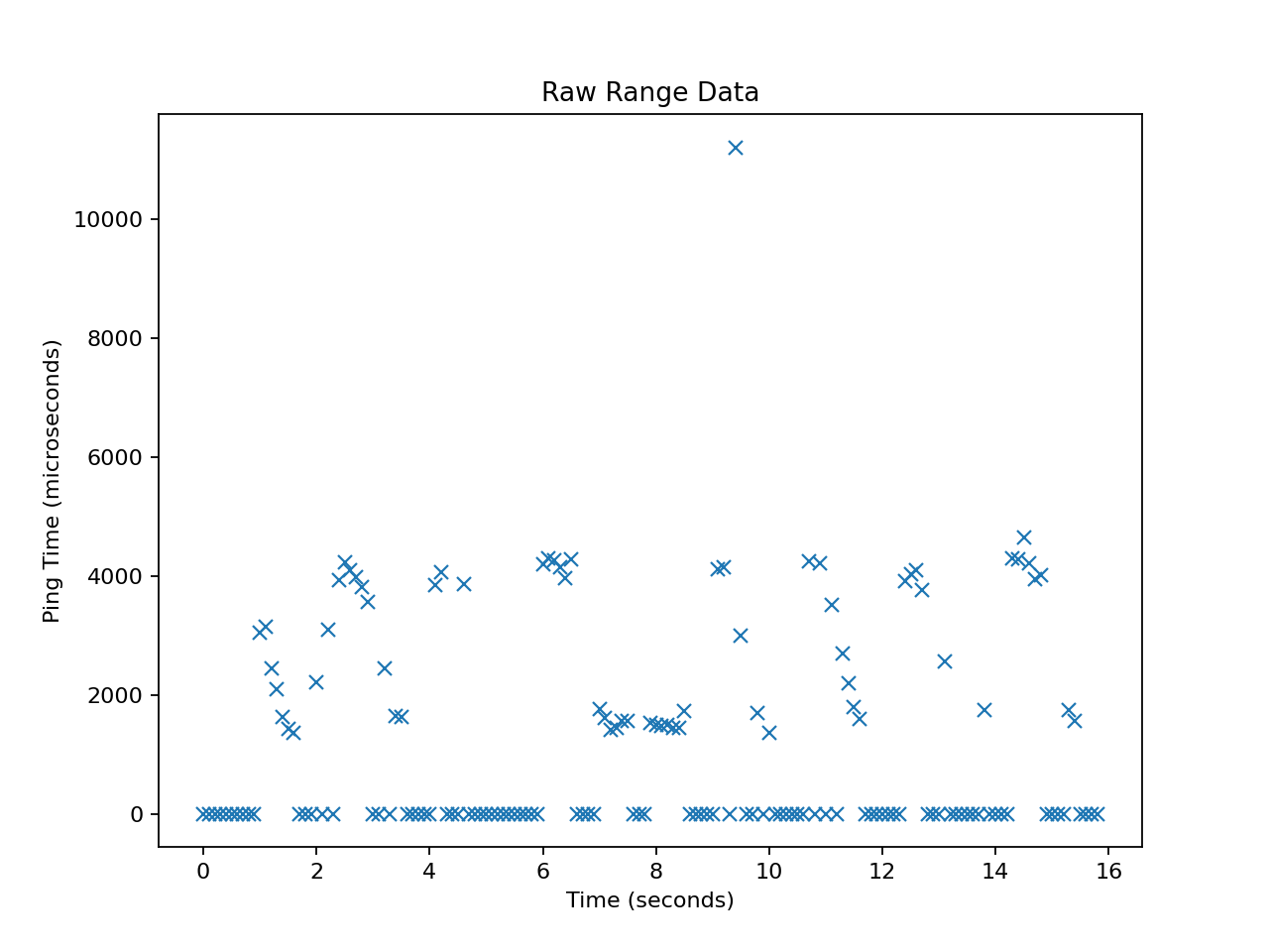
Unprocessed sonar range sensor data showing the round-trip ‘ping’ time in microseconds. The many zero readings denote the ‘no ping’ condition where the device failed to report an echo within the 11.8 millisecond limit. This can indicate a number of conditions: missing or weak echo, first echo surface farther than two meters away, specular reflection of ping away from device, or device malfunction.
Median of Three
A median filter is a non-linear smoothing filter intended to remove noisy outlier samples from a signal. For each sliding window of samples, the median value is calculated and used as the sample value. In a smooth signal, a single spurious measurement is likely to fall outside the cluster of samples in a given window and will not affect the result (unlike averaging techniques).
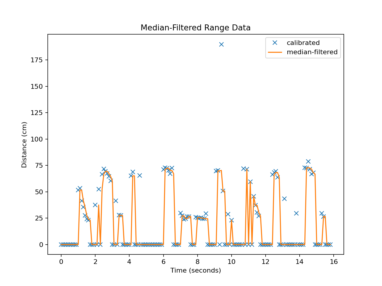
Result of applying median_3_filter() to the calculate the median of
each three-sample window. The filter notably removes the outlier at the
farthest range, but is not wide enough to affect the large number of zero
values. The ‘calibrated’ values are a linear rescaling of the unprocessed
ping times.
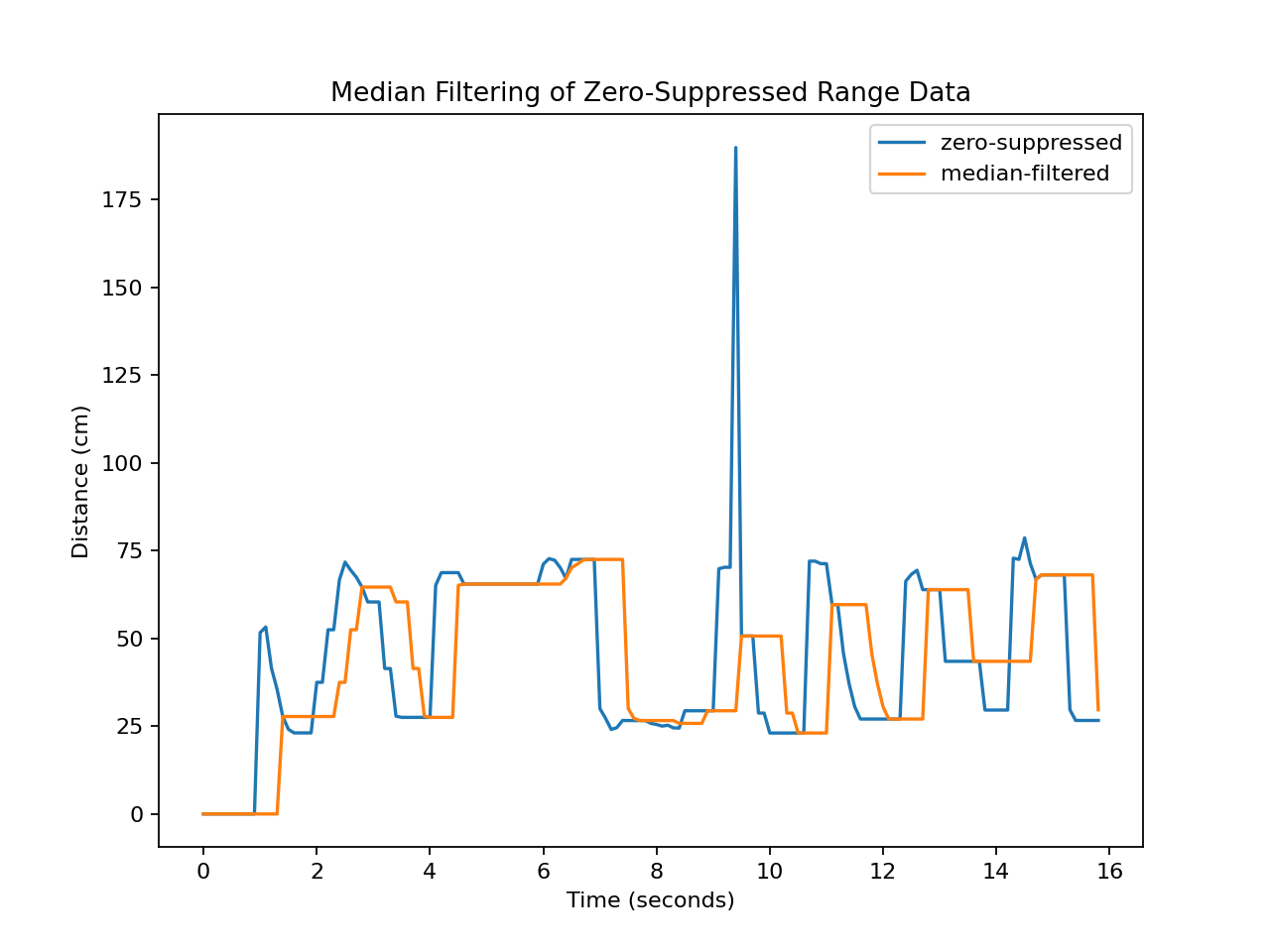
Smoothing
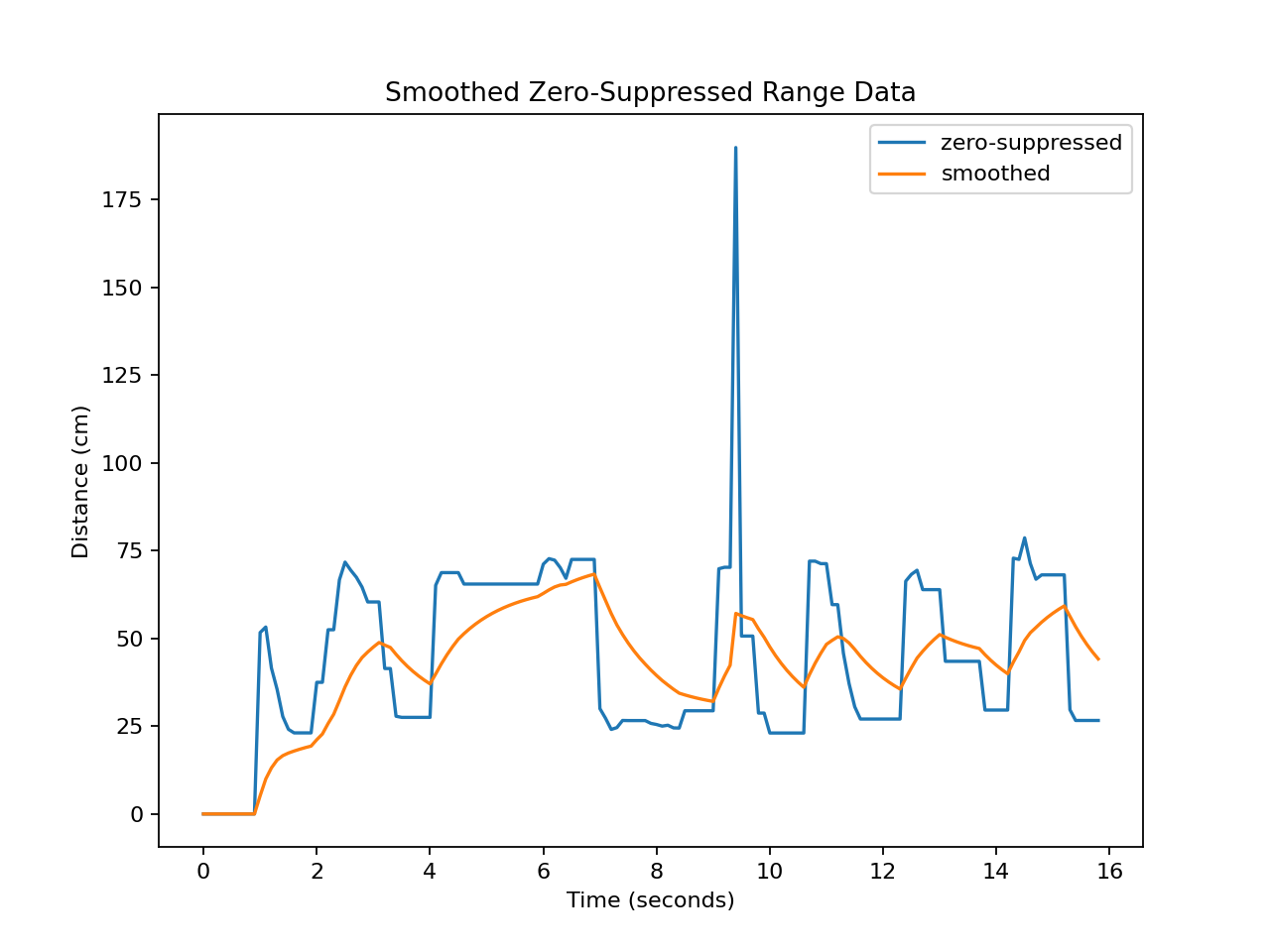
Result of applying a first-order smoothing filter to the zero-suppressed range data using a smoothing coefficient of 0.1.