Signal Processing Examples - CircuitPython

N.B. this is new and still being tested.

The following Python samples demonstrate several single-channel filters for processing sensor data. The filter functions are purely numeric operations and should work on any Python or CircuitPython system. This supports offline testing, as they can be debugged and evaluated on a normal desktop computer.

The code is written for clarity, not efficiency. In many cases significant speedup could result from using ulab or numpy to apply filters to sample vectors or matrices.

The source files can be browsed in raw form in the CircuitPython signals code folder. The files may be also downloaded in a single archive file as signals.zip.

linear.py

An important step in signal processing is applying a calibration transformation to translate raw values received from an analog to digital converter (ADC) into repeatable and meaningful units. For linear sensors this can be a two-parameter linear mapping which applies an offset and scaling. One convenient implementation is the map function.

map(x, in_min, in_max, out_min, out_max)

Map an input x from range (in_min, in_max) to range (out_min, out_max). This is a Python implementation of the Arduino map() function. Works on either integers or floating point.

constrain(x, a, b)

Constrains a number x to be within range (a, b). Python implementation of the Arduino constrain() function. N.B. included here for a convenience, but this is not a linear function.

# linear.py : platform-independent linear transforms
# No copyright, 2020-2021, Garth Zeglin.  This file is explicitly placed in the public domain.

def map(x, in_min, in_max, out_min, out_max):
    """Map an input x from range (in_min, in_max) to range (out_min, out_max).  This
    is a Python implementation of the Arduino map() function.  Works on either
    integers or floating point.
    """
    divisor = in_max - in_min
    
    if divisor == 0:
        return out_min
    else:
        return ((x - in_min) * (out_max - out_min) / divisor) + out_min

def constrain(x, a, b):
    """Constrains a number x to be within range (a, b).  Python implementation
    of the Arduino constrain() function."""
    return min(max(x, a), b)

statistics.py

class CentralMeasures

Object encapsulating a set of accumulators for calculating the mean, variance, min, and max of a stream of values. All properties are available as object attributes (i.e. instance variables).

# statistics.py : compute single-channel central measures in an accumulator
# No copyright, 2009-2021, Garth Zeglin.  This file is explicitly placed in the public domain.

import math

# CircuitPython lacks math.inf, here is a workaround:
try:
    inf_value = math.inf
except AttributeError:
    inf_value = math.exp(10000)


class CentralMeasures:
    def __init__(self):
        """Object to accumulate central measures statistics on a single channel of data."""

        self.samples = 0            # running sum of value^0, i.e., the number of samples
        self.total   = 0            # running sum of value^1, i.e., the accumulated total
        self.squared = 0            # running sum of value^2, i.e., the accumulated sum of squares
        self.minval  = inf_value    # smallest input seen
        self.maxval  = -inf_value   # largest input seen
        self.last = 0               # most recent input

        # computed statistics
        self.average  = 0           # mean value
        self.variance = 0           # square of the standard deviation

        return

    def update(self, value):
        """Apply a new sample to the accumulators and update the computed statistics.
        Returns the computed average and variance as a tuple."""
        self.total   += value
        self.squared += value * value

        if value < self.minval:
            self.minval = value

        if value > self.maxval:
            self.maxval = value

        self.samples += 1
        self.last = value

        # recalculate average and variance
        if self.samples > 0:
            self.average = self.total / self.samples

            if self.samples > 1:
                # The "standard deviation of the sample", which is only correct
                # if the population is normally distributed and a large sample
                # is available, otherwise tends to be too low:
                # self.sigma = math.sqrt((self.samples * self.squared - self.total*self.total) /
                #                         self.samples))

                # Instead compute the "sample standard deviation", an unbiased
                # estimator for the variance.  The standard deviation is the
                # square root of the variance.
                self.variance = ((self.samples * self.squared - self.total*self.total) /
                    (self.samples * (self.samples - 1)))

        return self.average, self.variance

hysteresis.py

Hysteresis is the behavior exhibited by a system with state dependent on its history. In physical systems it indicates the presence of hidden state, e.g., the magnetization of a material. In a filter it can provide useful non-linear behavior to discretize data or eliminate outliers.

class Hysteresis

Filter to quantize an input stream into a binary state. Dual thresholds are needed to implement hysteresis: the input needs to rise above the upper threshold to trigger a high output, then drop below the input threshold to return to the low output. One bit of state is required.

class Suppress

Fiilter to suppress a specific value in an input stream.

class Debounce

Filter to ‘debounce’ an integer stream by suppressing changes from the previous value until a specific new value has been observed a minimum number of times.

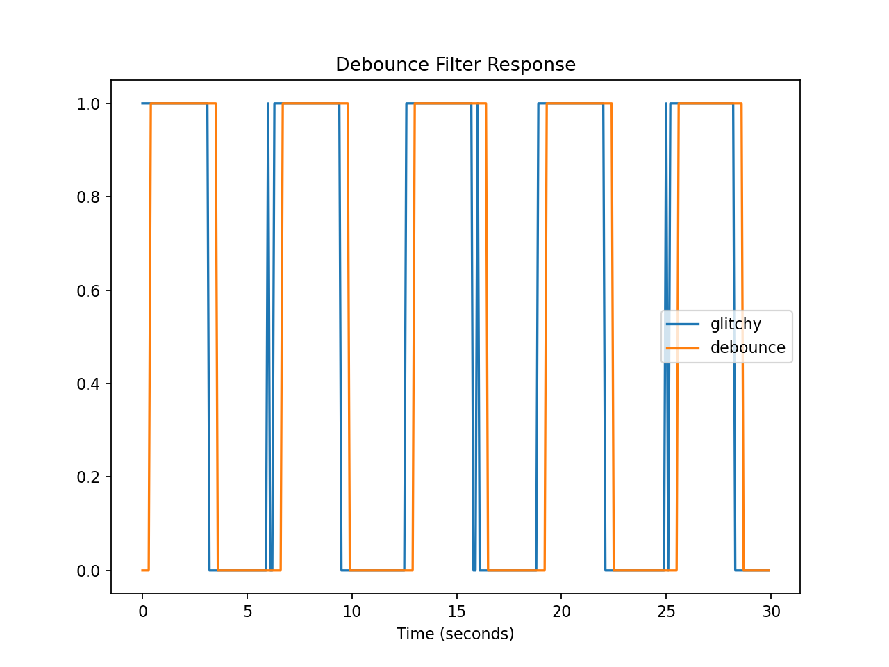
Time response of the debounce filter to a glitchy square wave. Note how the debounced signal ignores the extra transitions but is also slightly delayed.

# hysteresis.py : platform-independent non-linear filters

# No copyright, 2020-2011, Garth Zeglin.  This file is explicitly placed in
# the public domain.
#--------------------------------------------------------------------------------
class Hysteresis:
    def __init__(self, lower=16000, upper=48000):
        """Filter to quantize an input stream into a binary state.  Dual thresholds are
        needed to implement hysteresis: the input needs to rise above the upper
        threshold to trigger a high output, then drop below the input threshold
        to return to the low output.  One bit of state is required.
        """
        self.lower = lower
        self.upper = upper
        self.state = False

    def update(self, input):
        """Apply a new sample value to the quantizing filter.  Returns a boolean state."""
        if self.state is True:
            if input < self.lower:
                self.state = False
        else:
            if input > self.upper:
                self.state = True

        return self.state
    
#--------------------------------------------------------------------------------
class Suppress:
    def __init__(self, value=0):
        """Filter to suppress a specific value in an input stream."""
        self.suppress = value
        self.previous = None
        
    def update(self, input):
        if input != self.suppress:
            self.previous = input
        return self.previous

#--------------------------------------------------------------------------------
class Debounce:
    def __init__(self, samples=5):
        """Filter to 'debounce' an integer stream by suppressing changes from the previous value
        until a specific new value has been observed a minimum number of times."""

        self.samples = samples          # number of samples required to change        
        self.current_value = 0          # current stable value
        self.new_value = None           # possible new value        
        self.count = 0                  # count of new values observed

    def update(self, input):
        if input == self.current_value:
            # if the input is unchanged, keep the counter at zero            
            self.count = 0
            self.new_value = None
        else:
            if input != self.new_value:
                # start a new count
                self.new_value = input
                self.count = 1
            else:
                # count repeated changes
                self.count += 1
                if self.count >= self.samples:
                    # switch state after a sufficient number of changes
                    self.current_value = self.new_value
                    self.count = 0
                    self.new_value = None
                    
        return self.current_value

smoothing.py

class Smoothing

Filter to smooth an input signal using a first-order filter. One state value is required. The smaller the coefficient, the smoother the output.

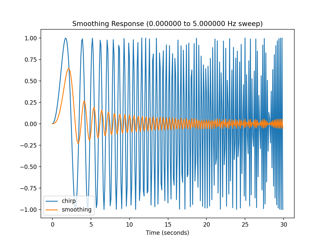
Time response of the smoothing filter to a ‘chirp’ frequency sweep. Note the effect is a soft low-pass filter, as compared to the Butterworth low-pass below.

class MovingAverage

Filter to smooth a signal by averaging over multiple samples. The recent time history (the ‘moving window’) is kept in an array along with a running total. The window size determines how many samples are held in memory and averaged together.

# smoothing.py : platform-independent first-order smoothing filter
# No copyright, 2020-2021, Garth Zeglin.  This file is explicitly placed in the public domain.

class Smoothing:
    def __init__(self, coeff=0.1):
        """Filter to smooth an input signal using a first-order filter.  One state value
         is required.  The smaller the coefficient, the smoother the output."""
        self.coeff = coeff
        self.value = 0

    def update(self, input):
        # compute the error between the input and the accumulator        
        difference = input - self.value

        # apply a constant coefficient to move the smoothed value toward the input        
        self.value += self.coeff * difference  

        return self.value

#--------------------------------------------------------------------------------
class MovingAverage:
    def __init__(self, window_size=5):
        """Filter to smooth a signal by averaging over multiple samples.  The recent
        time history (the 'moving window') is kept in an array along with a
        running total.  The window size determines how many samples are held in
        memory and averaged together.
        """
        self.window_size = window_size
        self.ring = [0] * window_size     # ring buffer for recent time history
        self.oldest = 0                   # index of oldest sample
        self.total  = 0                   # sum of all values in the buffer

    def update(self, input):
        # subtract the oldest sample from the running total before overwriting
        self.total = self.total - self.ring[self.oldest]
  
        # save the new sample by overwriting the oldest sample
        self.ring[self.oldest] = input

        # advance to the next position, wrapping around as needed
        self.oldest += 1
        if self.oldest >= self.window_size:
            self.oldest = 0

        # add the new input value to the running total
        self.total = self.total + input

        # calculate and return the average
        return self.total / self.window_size

median.py

class MedianFilter

Non-linear filter to reduce signal outliers by returning the median value of the recent history. The window size determines how many samples are held in memory. An input change is typically delayed by half the window width. This filter is useful for throwing away isolated outliers, especially glitches out of range.

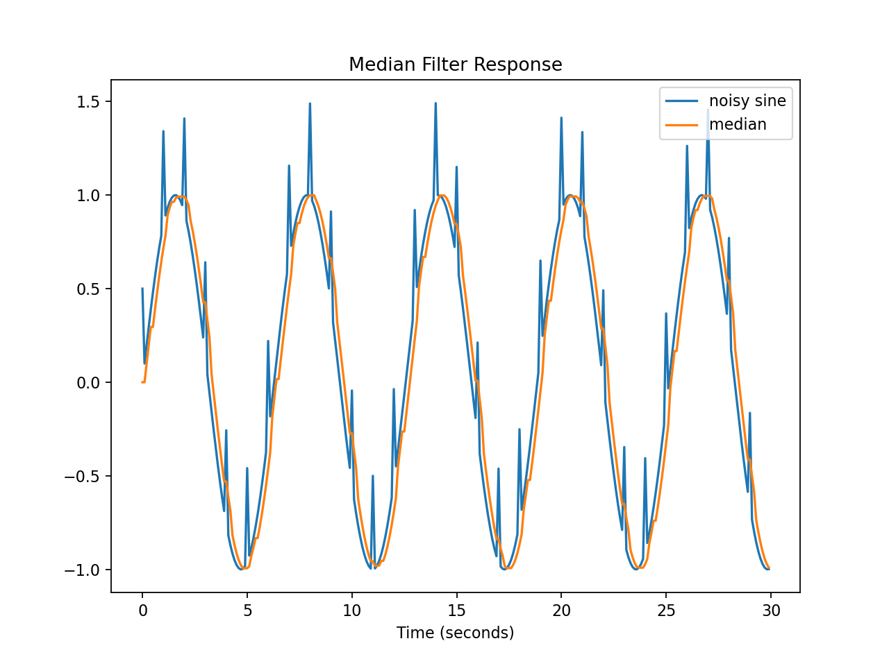
Time response of the median filter to a sine wave with added spikes. Note how the isolated glitches have little effect.

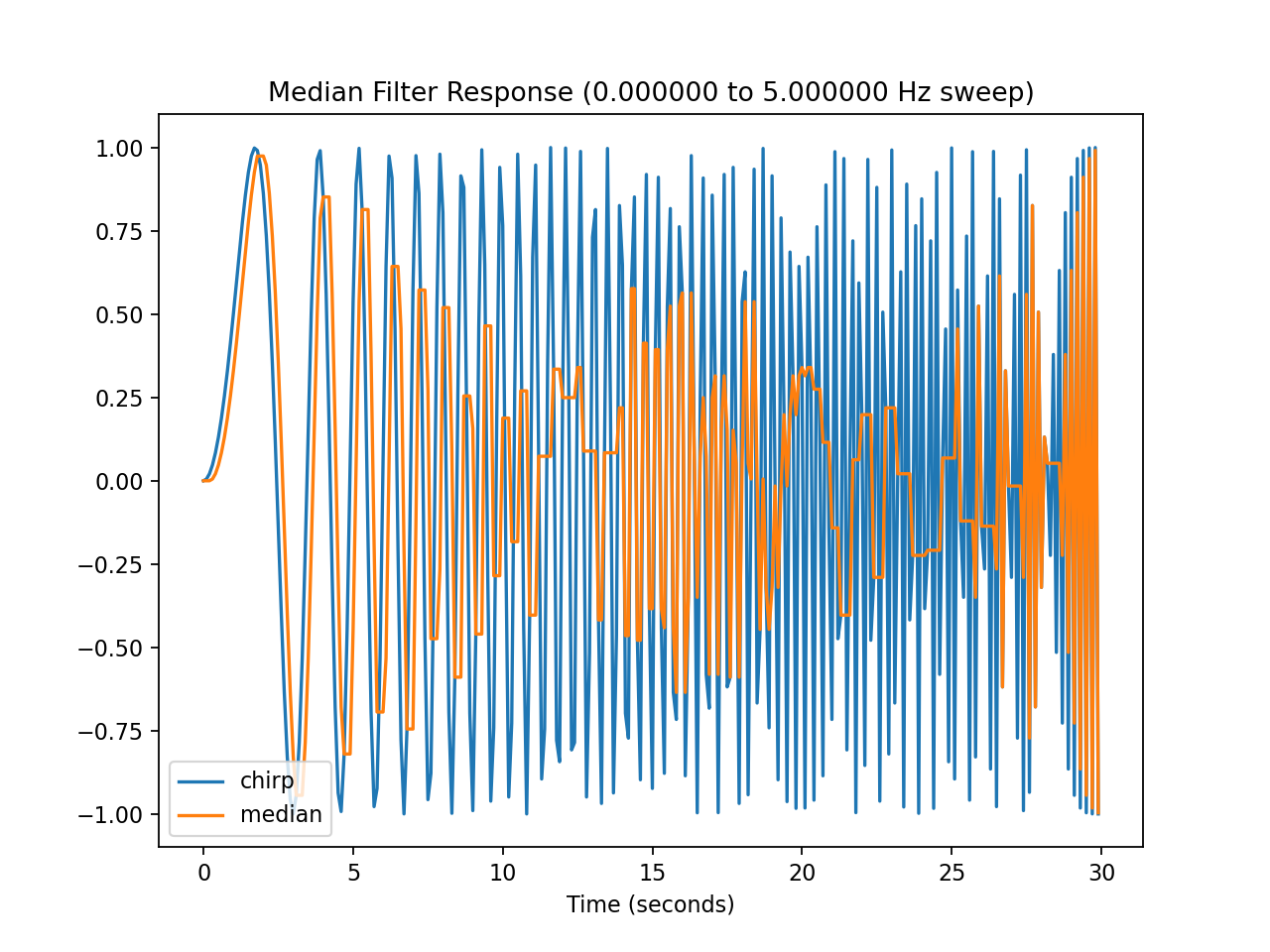
Time response of the median filter to a ‘chirp’ frequency sweep. The response is erratic; this is not a linear filter.

# median.py : platform-independent median filter
# No copyright, 2020-2021, Garth Zeglin.  This file is explicitly placed in the public domain.

class MedianFilter:
    def __init__(self, window_size=5):
        """Non-linear filter to reduce signal outliers by returning the median value
        of the recent history.  The window size determines how many samples
        are held in memory.  An input change is typically delayed by half the
        window width.  This filter is useful for throwing away isolated
        outliers, especially glitches out of range.
        """
        self.window_size = window_size
        self.ring = [0] * window_size     # ring buffer for recent time history
        self.oldest = 0                   # index of oldest sample

    def update(self, input):
        # save the new sample by overwriting the oldest sample
        self.ring[self.oldest] = input
        self.oldest += 1
        if self.oldest >= self.window_size:
            self.oldest = 0

        # create a new sorted array from the ring buffer values
        in_order = sorted(self.ring)

        # return the value in the middle
        return in_order[self.window_size//2]

biquad.py

class BiquadFilter

General IIR digital filter using cascaded biquad sections. The specific filter type is configured using a coefficient matrix. These matrices can be generated for low-pass, high-pass, and band-pass configurations.

The file also contains filter matrices automatically generated using filter_gen.py and the SciPy toolkit. In general you will need to regenerate the filter coefficients for your particular application needs. The sample filter responses are shown below.

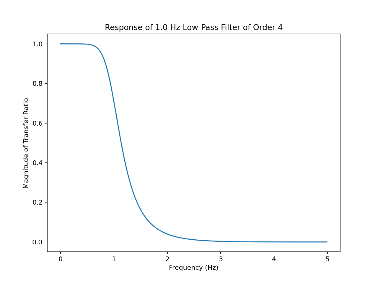
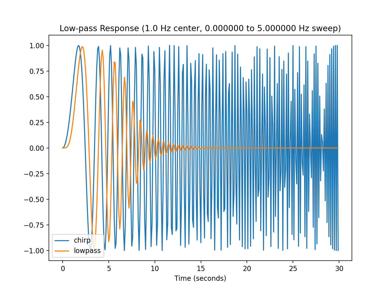
On the left is the low-pass filter signal transfer ratio as a function of frequency. Please note this is plotted on a linear scale for clarity; on a logarithmic scale (dB) the rolloff slope becomes straight. On the right is the low-pass filter time response to a ‘chirp’ frequency sweep.

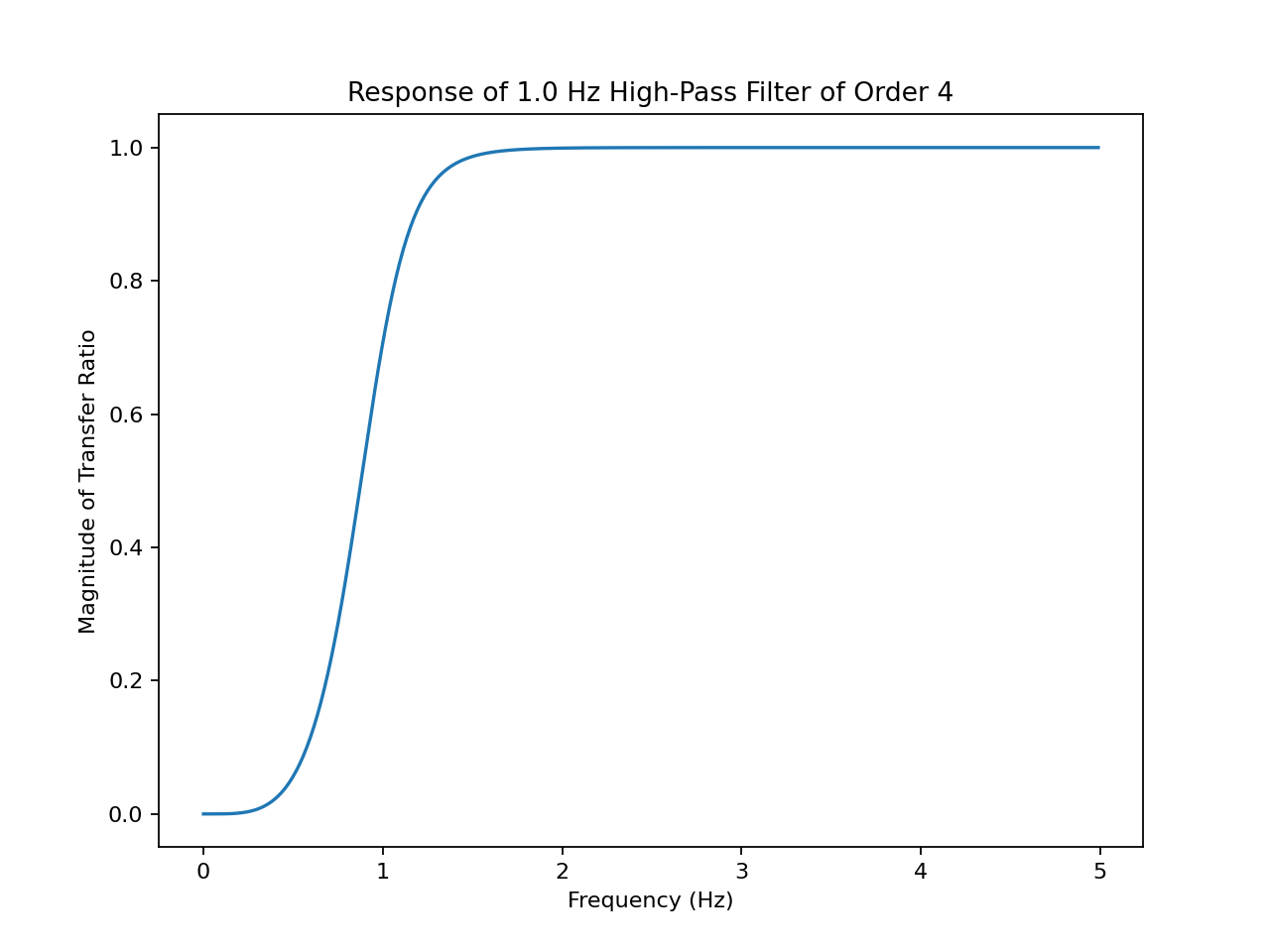
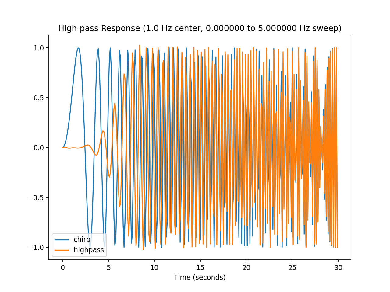
On the left is the high-pass filter signal transfer ratio as a function of frequency, on the right is the time response.

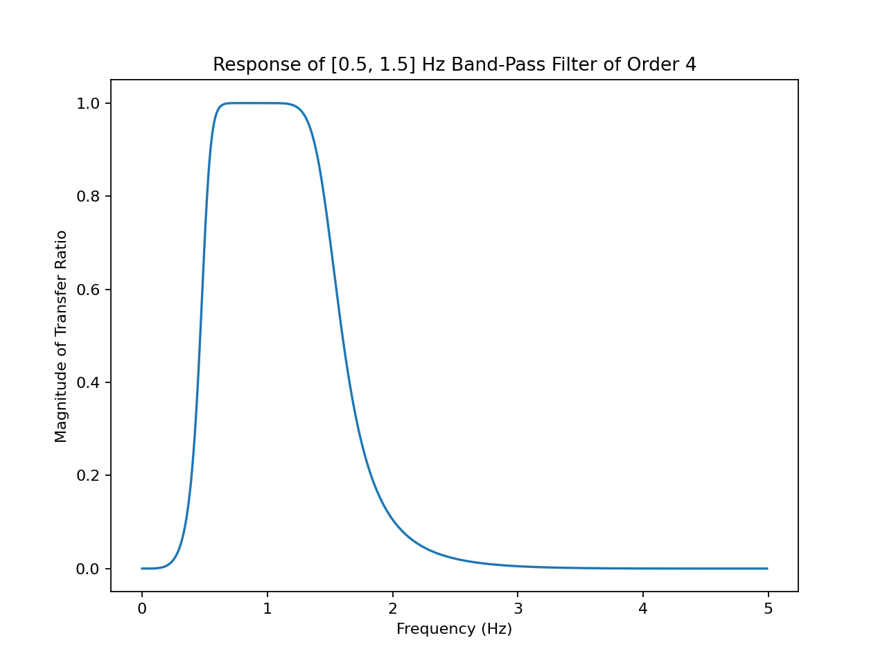
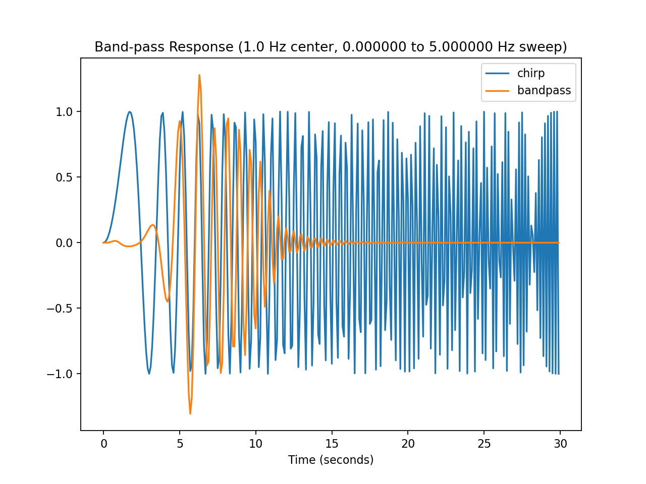
On the left is the band-pass signal transfer ratio as a function of frequency, on the right is the time response.

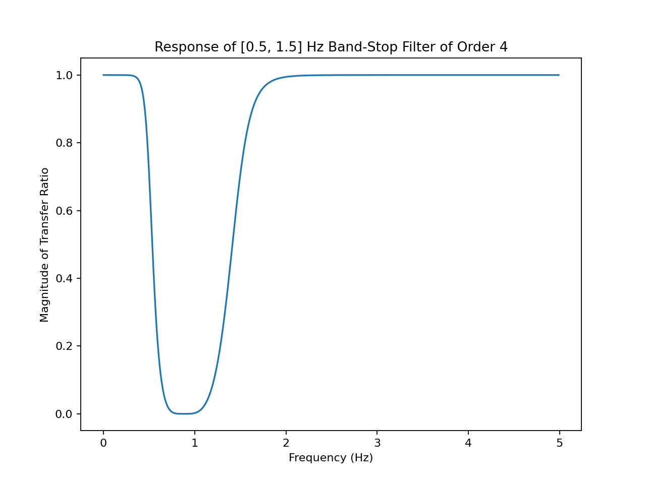
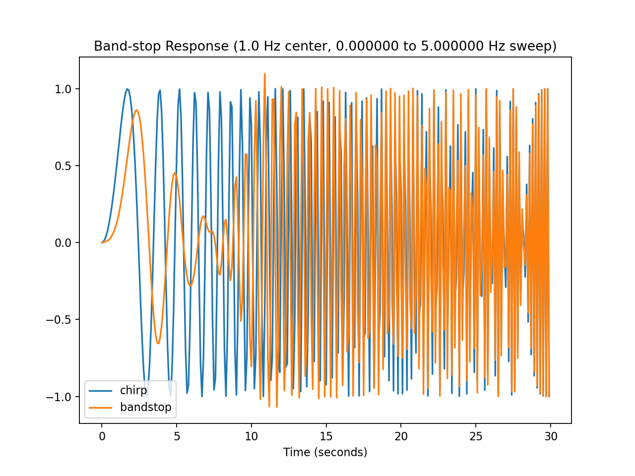
On the left is the band-stop signal transfer ratio as a function of frequency, on the right is the time response.

# biquad.py : digital IIR filters using cascaded biquad sections generated using filter_gen.py.

#--------------------------------------------------------------------------------
# Coefficients for a low-pass Butterworth IIR digital filter with sampling rate
# 10 Hz and corner frequency 1.0 Hz.  Filter is order 4, implemented as
# second-order sections (biquads).
# Reference: https://docs.scipy.org/doc/scipy/reference/generated/scipy.signal.butter.html

low_pass_10_1 = [[[1.0,       -1.04859958, 0.29614036],   # A coefficients, first section
                  [0.00482434, 0.00964869, 0.00482434]],  # B coefficients, first section
                 [[1.0,       -1.32091343, 0.63273879],   # A coefficients, second section
                  [1.0,        2.0,        1.0]]]         # B coefficients, second section

#--------------------------------------------------------------------------------
# Coefficients for a high-pass Butterworth IIR digital filter with 
# sampling rate: 10 Hz and corner frequency 1.0 Hz.
# Filter is order 4, implemented as second-order sections (biquads).

high_pass_10_1 = [[[1.0,        -1.04859958, 0.29614036],
                   [0.43284664, -0.86569329, 0.43284664]],
                  [[1.0,        -1.32091343, 0.63273879],
                   [1.0,        -2.0,        1.0]]]

#--------------------------------------------------------------------------------
# Coefficients for a band-pass Butterworth IIR digital filter with sampling rate
# 10 Hz and pass frequency range [0.5, 1.5] Hz.  Filter is order 4, implemented
# as second-order sections (biquads).
band_pass_10_1 = [[[1.0,        -1.10547167, 0.46872661],
                   [0.00482434,  0.00964869, 0.00482434]],
                  [[1.0,        -1.48782202, 0.63179763],
                   [1.0,        2.0,         1.0]],
                  [[1.0,        -1.04431445, 0.72062964],
                   [1.0,        -2.0,        1.0]],
                  [[1.0,        -1.78062325, 0.87803603],
                   [1,          -2.0,        1.0]]]

#--------------------------------------------------------------------------------
# Coefficients for a band-stop Butterworth IIR digital filter with
# sampling rate: 10 Hz and exclusion frequency range [0.5, 1.5] Hz.
# Filter is order 4, implemented as second-order sections (biquads).

band_stop_10_1 = [[[1.0,        -1.10547167, 0.46872661],
                   [0.43284664, -0.73640270, 0.43284664]],
                  [[1.0,        -1.48782202, 0.63179763],
                   [1.0,        -1.70130162, 1.0]],
                  [[1.0,        -1.04431445, 0.72062964],
                   [1.0,        -1.70130162, 1.0]],
                  [[1.0,        -1.78062325, 0.87803603],
                   [1.0,        -1.70130162, 1.0]]]

#--------------------------------------------------------------------------------
class BiquadFilter:
    def __init__(self, coeff=low_pass_10_1):
        """General IIR digital filter using cascaded biquad sections.  The specific
        filter type is configured using a coefficient matrix.  These matrices can be
        generated for low-pass, high-pass, and band-pass configurations.
        """
        self.coeff = coeff                                 # coefficient matricies
        self.sections = len(self.coeff)                    # number of biquad sections in chain
        self.state = [[0,0] for i in range(self.sections)] # biquad state vectors
        
    def update(self, input):
        # Iterate over the biquads in sequence.  The accum variable transfers
        # the input into the chain, the output of each section into the input of
        # the next, and final output value.
        accum = input        
        for s in range(self.sections):
            A = self.coeff[s][0]
            B = self.coeff[s][1]
            Z = self.state[s]
            x     = accum   - A[1]*Z[0] - A[2]*Z[1]
            accum = B[0]*x  + B[1]*Z[0] + B[2]*Z[1]
            Z[1] = Z[0]
            Z[0] = x

        return accum

demo.py

This following script applies all the sample filters to an analog sample stream. This file should be copied into the top-level folder as code.py, and the individual filter samples under their own names so they may be loaded as modules.

# demo.py

# Raspberry Pi Pico - Signal Processing Demo

# Read an analog input with the ADC, apply various filters, and print filtered
# data to the console for plotting.

# Import CircuitPython modules.
import board
import time
import analogio
import digitalio

# Import every filter sample.  These files should be copied to the top-level
# directory of the CIRCUITPY filesystem on the Pico.

import biquad
import hysteresis
import linear
import median
import smoothing
import statistics

#---------------------------------------------------------------
# Set up the hardware.

# Set up an analog input on ADC0 (GP26), which is physically pin 31.
# E.g., this may be attached to photocell or photointerrupter with associated pullup resistor.
sensor = analogio.AnalogIn(board.A0)

#---------------------------------------------------------------
# Initialize filter objects as global variables.

stats        = statistics.CentralMeasures()
hysteresis   = hysteresis.Hysteresis(lower=0.25, upper=0.75)
average      = smoothing.MovingAverage()
smoothing    = smoothing.Smoothing()
median       = median.MedianFilter()
lowpass      = biquad.BiquadFilter(biquad.low_pass_10_1)
highpass     = biquad.BiquadFilter(biquad.high_pass_10_1)
bandpass     = biquad.BiquadFilter(biquad.band_pass_10_1)
bandstop     = biquad.BiquadFilter(biquad.band_stop_10_1)

# Collect all the filters in a list for efficient multiple updates.

all_filters = [ stats, hysteresis, average, smoothing, median,
                lowpass, highpass, bandpass, bandstop, ]

#---------------------------------------------------------------
# Run the main event loop.

# Use the high-precision clock to regulate a precise *average* sampling rate.
sampling_interval  = 100000000           # 0.1 sec period of 10 Hz in nanoseconds
next_sample_time   = time.monotonic_ns()

while True:
    # read the current nanosecond clock
    now = time.monotonic_ns()
    if now >= next_sample_time:
        # Advance the next event time; by spacing out the timestamps at precise
        # intervals, the individual sample times may have 'jitter', but the
        # average rate will be exact.
        next_sample_time += sampling_interval
        
        # Read the sensor once per sampling cycle.
        raw = sensor.value

        # Apply calibration to map integer ADC values to meaningful units.  The
        # exact scaling and offset will depend on both the individual device and
        # application.
        calib  = linear.map(raw, 59000, 4000, 0.0, 1.0)

        # Pipe the calibrated value through all the filters.
        filtered = [filt.update(calib) for filt in all_filters]

        # Selectively report results for plotting.
        # print((raw, calib))                            # raw and calibrated input signal
        # print((calib, filtered[0][0], filtered[0][1])) # calibrated, average, variance
        # print((calib, 1*filtered[1], filtered[2]))     # calibrated, thresholded, moving average
        print((calib, filtered[3], filtered[4]))         # calibrated, smoothed, median-filtered
        # print((calib, filtered[5], filtered[6]))       # calibrated, low-pass, high-pass
        # print((calib, filtered[7], filtered[8]))       # calibrated, band-pass, band-stop

Development Tools

The development of these filters involves several other tools:

• A Python script for generating digital filters using SciPy: filter_gen.py

• A Python matplotlib script for generating figures from the test data: generate_plots.py

The Python scripts use several third-party libraries:

• SciPy: comprehensive numerical analysis; linear algebra algorithms used during filter generation

• Matplotlib: plotting library for visualizing data

For more information on filters:

• https://en.wikipedia.org/wiki/Digital_biquad_filter

• https://en.wikipedia.org/wiki/Median_filter