The universe can be modeled from springs. Nearly every solid material can be thought of as a collection of particles which are attached to each other by elastic forces.
From Isaac Newton (1686), we know his second law of motion, that F = ma.
This states that in general, force is proportional to mass times acceleration.
From Robert Hooke (1678), we know the spring law, F = -Kx.
This states that the force applied by a spring, is proportional (by some constant K) to its distention x (amount of stretch or compression). The minus sign tells us that the spring’s “restorative force” happens in the opposite direction.
To take an example, if you stretch a spring (which is rigidly fixed at one end) one centimeter to the east, it will apply a restoring force towards the west. If you stretch it two centimeters eastward, it will apply a westerly force which is twice as strong.
Because F = ma and F = -kx, we can derive that ma = -kx. Interestingly, this is actually a “second-order differential equation” — which describes a relationship between a particle’s position, x, and its acceleration (or the rate of change of the rate of change of its position), a. The solution to such equations always take the form of an “exponentially damped cosinusoid”, in what is called damped harmonic motion:
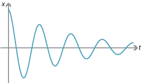
Pleasingly, this exactly captures the movement of a spring over time: it wiggles back and forth, gradually losing energy due to friction. Depending on the amount of damping, the spring may be very wiggly, or not. We use terms like overdamped and underdamped to describe this:
The constant K is the “spring constant” which is unique for each material. When the value of K is high, the material is stiff, snappy or brittle. When K is low, the material is soft, flexible, stretchy. (High values of K will expose the limits of Euler integration, our current numerical method for solving springs here; if K is too high, the simulation will “explode”. We’ll let you discover that…). You can find the value of K in the code samples below. Good values for our solver are in the range of 0.01 to 0.5; try using 0.1 to get started.
There is also a damping factor in our particles which describes how much energy they retain after each frame of animation. A value of 0.96 is fine to get started (meaning, they lose 4% of their energy each frame). Under no circumstances should you ever set this higher than 1.0! Lower values (e.g. 0.7, 0.5, etc.) will cause overdamping.
Springs 1 (Simple)
Here, two particles are connected to each other by a spring. Pulling one away from the other, causes the spring to exert an elastic restorative force on each.
springs-simple.js
When particles are connected by rigid elements in a triangle, we have the fundamental element of truss structures. All architects know this. (The following simulation also has a gravity force added in to the particles, so that they are affected both by gravity and by spring forces.)
springs-triangle.js
It’s possible to “fix” one or more particles to a rigid location. It is as if one particle were attached to something too large to move:
springs-fixed.js
Springs 2 (Rope, with and without Gravity)
We can connect multiple particles into a rope. A for() loop has been used to connect each particle to the next one. Here we see the basic code structure we will be using: an array of particles, and an array of springs which (selectively) connects certain ones among them:
springs-rope.js
Here is the same example, but with a gravity force added in. Architects will readily recognize that the simulation is able to achieve the well-known catenary curve.
springs-rope-gravity.js
Springs 3 (Blob)
In this example, particles are placed around the perimeter of a circle. Then springs are used to connect each one to its neighbor. All of particles are also connected by a spring to a single central particle, like spokes of a wheel. I have taken the liberty of decorating this set of particles with a closed Bezier curve that stitches through them all:
springs-wheel.js
In this example, particles are placed around the perimeter of a circle. Then springs are used to connect (some of) them. Specifically, particles are connected to their neighbors, and some of their other nearby neighbors as well. The result is a kind of bouncy bag:
springs-blob.js
Springs 4 (Big Square Mesh)
Here is a classic mesh. Just as in real life, for proper rigidity, we have to connect elements diagonally, or else the structure will not have integrity and will collapse. The code for doing so is (slightly) tricky.
springs-mesh1.js
Springs 5 (Auto-Bouncy Mesh)
We can grab one of the particles and move it automatically. Here one particle is being moved by a combination of sinusoidal and Perlin-noise forces. The rest of the mesh accommodates. (Note that this example is not interactive.)
springs-mesh2
Springs 6 (Narrow Truss)
Here is a narrow truss which imitates a bottom-feeding worm:
springs-truss.js