Category: Uncategorized

/* Evan Stuhlfire
 * estuhlfi@andrew.cmu.edu Section B
 * Project-07: Composition with Curves 
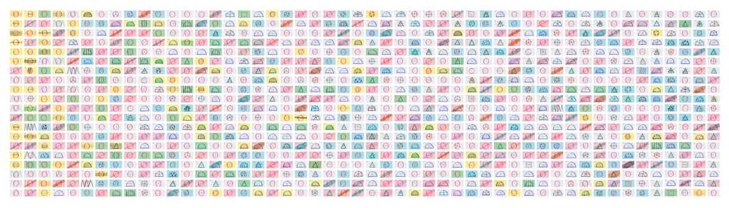
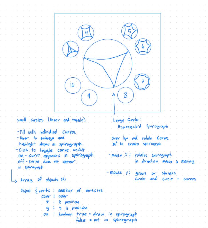
 * Hypocycloid Spirograph */

var rAngle = 30; // rotation angle
var rotation = 0; // degrees of rotation
var maxShapes = 8;
var shape = []; // array of shapes

function setup() {
    createCanvas(480, 480);
    background(250);
    // fill array of objects with default shapes
    createShapes();
}

function draw() {
     // redraw background
    background(250);
    stroke(200);

    // map the mouseX position to a circle for rotation radians
    var xRot = map(mouseX, 0, width, 0, TWO_PI);
    // map the mouseY to half the height to size the shape 
    var my = map(mouseY, 0, height, 50, height/2);
    // r is based on the y position and becomes the radius of the circle
    var r = constrain(my, 100, height/2 - 75);

    // add text to canvas
    addText();

    push(); // store settings
    // translate origin to center
    translate(width/2, height/2);

    // draw the small circles and their curves
    for(var s = 0; s < shape.length; s++) {
        drawSmallShapes(s, height/2 - 25);
    }


    // rotate the canvas based on the mouseX position
    rotate(xRot);
    circle(0, 0, 2 * r);
    // loop over array of shape objects
    for(var s = 0; s < shape.length; s++) {
        // drawSmallShapes(s, maxr);
        // reset degrees of rotation for each shape
        rotation = 0; 
        if(shape[s].on == true){
            // draw the curve in spirograph, 4 times for curve rotation
            for(var i = 0; i < 4; i++) {
                // rotation canvas, start at 0
                rotate(radians(rotation));
                rotation = rAngle;
                drawCurves(shape[s].verts, r, shape[s].color);
            }            
        }
    }
    pop(); // restore settings
}

function mousePressed() {
    // when a shape is clicked it is added or removed
    // from the spirograph, toggles like a button

    // map the mouse position to the translated canvas
    var mx = map(mouseX, 0, width, -240, 240);
    var my = map(mouseY, 0, height, -240, 240);

    // loop through shapes to see if clicked
    for(var i = 0; i < shape.length; i++) {
        var d = dist(shape[i].px, shape[i].py, mx, my);

        // check distance mouse click from center of a shape
        if(d <= shape[i].radius){
            // if on, set to false
            if(shape[i].on == true) {
                shape[i].on = false;  
            } else {
                // if on = false, set true
                shape[i].on = true;
            }
        }
    }
}

function addText() {
    // Add text to canvas
    fill(shape[0].colorB);
    strokeWeight(.1);
    textAlign(CENTER, CENTER);

    // title at top
    textSize(20);
    text("Hypocycloid", width/2, 8);
    text("Spirograph", width/2, 30);
    // directions at bottom
    textSize(10);
    text("Click the circles to toggle curves on or off. Reload for different pen colors.", 
        width/2, height - 5);

    noFill();
    strokeWeight(1);
}

function createShapes() {
    var vCount = 3; // start shapes with 3 verticies
    var sOn = true; // default first shape to show in spirograph
    var angle = 30;
    var shapeRad = 35;

    // create array of shape objects
    for(var i = 0; i < maxShapes; i++) {
        shape[i] = new Object();

        // set object values
        shape[i].verts = vCount;
        // generate random color Bright and Dull for each
        var r = random(255);
        var g = random(255);
        var b = random(255);

        shape[i].colorB = color(r, g, b, 255); // Bright color
        shape[i].colorM = color(r, g, b, 80); // Muted faded color
        shape[i].color = shape[i].colorM;
        shape[i].angle = angle;
        shape[i].px = 0;
        shape[i].px = 0;
        shape[i].radius = shapeRad;
        shape[i].on = sOn;

        // default shapes to not display in spirograph
        sOn = false;      
        vCount++;
        angle += 30;
        if (angle == 90 || angle == 180 || angle == 270) {
            angle += 30;
        }
    }
}

function drawSmallShapes(s, r) {
    // calculate the parametric x and y
    var px = r * cos(radians(shape[s].angle));
    var py = r * sin(radians(shape[s].angle));
    shape[s].px = px;
    shape[s].py = py;

    // map the mouse position to the translated canvas
    var mx = map(mouseX, 0, width, -240, 240);
    var my = map(mouseY, 0, height, -240, 240);

    // check if mouse is hovering over small circle
    var d = dist(shape[s].px, shape[s].py, mx, my);
    if(d <= shape[s].radius) {
        // hovering, make bigger, make brighter
        var hover = 1.25;
        shape[s].color = shape[s].colorB;
    } else {
        // not hovering, make normal size, mute color
        var hover = 1;
        shape[s].color = shape[s].colorM;
    }

    // check if shape is appearing in spriograph
    if(shape[s].on == true) {
        var c = shape[s].colorB; // bright
    } else {
        var c = shape[s].colorM; // muted
    }

    push();
    // move origin to little circle center
    translate(px, py);
    stroke(c); // set color from object
    strokeWeight(2);

    circle(0, 0, shape[s].radius * 2 * hover); // draw little circle
    // draw the curve in the little circle
    drawCurves(shape[s].verts, shape[s].radius * hover, c)
    pop();
}

function drawCurves(n, r, c) {
    // n = number of shape verticies, r = radius, c = color
    // number of vertices for drawing with beginShape
    var nPoints = 50;

    beginShape();
    for(var i = 0; i < nPoints; i++) {
        // map the number of points to a circle
        var t = map(i, 0, nPoints, 0, TWO_PI); // t = theta
        // fit the shape to the radius of the circle
        var value = r/n;
        // calculate hypocycloid at a different number of cusps.
        var px = value * ((n - 1) * cos(t) - cos((n - 1) * t));
        var py = value * ((n - 1) * sin(t) + sin((n - 1) * t)); 
    
        vertex(px, py); // add a vertex to the shape
    }
    noFill();
    stroke(c);
    strokeWeight(1);
    endShape(CLOSE); // close shape
}

// Zoe Lin (ID: youlin)
// Section B

var nPoints = 80;
var angle;
var x, y, theta;
var r, g, b;

function setup() {
  createCanvas(480, 480);
}

function draw() {
  r = map(mouseX, 0, width, 0, 20); //draws bg color based on mouse pos
  g = map(mouseY, 0, height, 0, 20);
  b = map(mouseX, 0, height, 0, 20);
  background(r, g, b);
  noFill();
  stroke(130);
  translate(width/2, height/2);
  moddedeEpitrochoid(); //draws first geometry at center
  rotate(HALF_PI); //draws second at an angle
  moddedeEpitrochoid();
  hypotrochoid(); 
  rotate(PI / 3); //repeat at third angle
  moddedeEpitrochoid();
  hypotrochoid();

function moddedeEpitrochoid() {
    var a = 85; //angle
    var h = constrain(mouseY / 10, 0, 100); //limits geometry size
    var mouse = mouseX / 70;
    
    beginShape();
    for (var i = 0; i < nPoints; i++) {
        theta = map(i, 0, nPoints, 0, TWO_PI);
        //modified formula for epitrochoid
        x = (a+a/2) * sin(theta) - cos(mouse + theta * (a + a/2) / a/2) * h;
        y = (a+a/2) * cos(theta) - sin(mouse + theta * (a + a/2) / a/2) * h;
        vertex(x, y);
        vertex(y, x); //layers vertexes, draws 2d geometry
    }
    endShape();
 }
  strokeWeight(0.25);
}

function hypotrochoid() { 
    var h = constrain(mouseX / 100, 205, height); //contrains geometry size
    var a = map(mouseX, 0, width, 25, 15); //maps mouse pos to desired angle
    var b = map(mouseY, 0, height, 0, 15);
    beginShape();
      for (var i = 0; i < nPoints-15; i ++) {
        var theta2 = map(i, 0, width/2, 0, 50);
        //hypotrochoid formula
        x = (a - b) * cos(theta2) + h * sin((a - b) * theta2);
        y = (a - b) * sin(theta2) - h * cos((a - b) * theta2);
        vertex(x, y);
      }
    endShape();
}