//Alicia Kim
//yoonbink@andrew.cmu.edu
//Section B

var nPoints = 100;
var r;

function setup() {
    createCanvas(480, 480);
    background(220);

    r=0;


}

function draw() {

// gradient background (adapted from my project 6)
    for(var j=0; j<height; j+=1) {
        stroke(lerpColor(color(127,255,212) ,color(255,253,208),j/height));
        line(0,j,width,j);
    }

    noStroke();

    push();
    translate (width/2, height/2);

    noFill();
    if (r<=15){
        r+=0.17;
    }
    else{r=0}
    drawHeart2(r);
    drawDevil();
    pop();

    drawHeart1();
}

function drawDevil() {
    // https://mathworld.wolfram.com/DevilsCurve.html
    // adapted from drawCranoid example from Wk 7 Deliverable example


    var x;
    var y;


    fill(250,250,210);
    beginShape();
    for (var i = 0; i < nPoints; i++) {


        var a = constrain((mouseX / width), -16.0, 16.0);
        var b = constrain((mouseY / height), -16.0, 16.0);
        var t = map(i, 0, nPoints, 0, TWO_PI);


        x = 100*cos(t)*sqrt((sq(a)*sq(sin(t))-(sq(b)*sq(cos(t)))/(sq(sin(t))-sq(cos(t)))));
        y = 100*sin(t)*sqrt((sq(a)*sq(sin(t))-(sq(b)*sq(cos(t)))/(sq(sin(t))-sq(cos(t)))));
        vertex(x, y);
    }
    endShape();
}

//cursor  heart
function drawHeart1(){

    var x2;
    var y2;

    fill(250);
    beginShape();
    for (var j = 0; j < nPoints; j++) {

        var t2 = map(j, 0, nPoints, 0, TWO_PI);


        x2 = mouseX+2*16*pow(sin(t2),3);
        y2 = 2*(13*cos(t2)-5*cos(2*t2)-2*cos(3*t2)-cos(4*t2));
        y2= mouseY-y2
        vertex(x2, y2);
    }
    endShape();
}

//background heart
function drawHeart2(r){

    var x3;
    var y3;
    // var r;
    fill(173,216,230);
    beginShape();
    // r=10;
    // r+=1;

    for (var j = 0; j < nPoints; j++) {

        var t2 = map(j, 0, nPoints, 0, TWO_PI);


        x3 = r*16*pow(sin(t2),3);
        y3 = -r*(13*cos(t2)-5*cos(2*t2)-2*cos(3*t2)-cos(4*t2));

        vertex(x3, y3);
    }
    endShape();
}Category: SectionB
Looking Outwards 07: Information Visualization
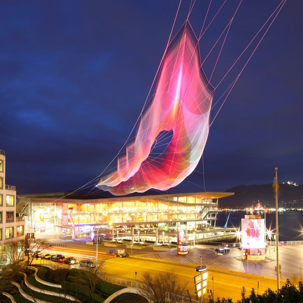
I am inspired by the project, Unnumbered Sparks by Aaron Koblin. This interactive sculpture installation is a combination of art and technology based on custom software.
Basically, the sculpture is made up of a complex matrix of hand and machine-made knots and braided fiber, and it’s spanned between the city’s existing architectures. To create a geometric and structural design for the rope network, the artist utilized a custom software, implementing an “adaptive form finding” algorithm. He also used the custom 3D software by Autodesk to model the sculpture and test its feasibility by exploring density, shape, and scale in greater detail. What makes this giant aerial netted sculpture special and admirable is the dynamic interaction between visitors and the artwork; The work visualizes visitors’ physical gestures on mobile devices in real-time through multi-colored light projection on the sculpture. The creator’s artistic sensibilities are manifested in his pattern design of the structural ropes and the aesthetic installation of it that well blends into the city environment.
http://www.aaronkoblin.com/project/unnumbered-sparks/
Looking Outward 07 / Dr. Lev Manovich
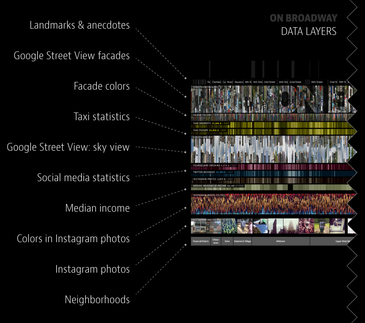
This week I’m looking at the work of Dr. Lev Manovich, particularly his ‘On Broadway’ project which was inspired by Edward Ruscha’s 1966 unfolding photo book titled ‘Every Building on the Sunset Strip’.
To gather data, Manovich and his team chose anchor points along Broadway to create 100 meter wide ‘slices’ which were combined to create a spine-like shape. The coordinates of the shape were then used to filter all of the data gathered, including Instagram posts made within each 100 meter section, Google images, Twitter posts, taxi pickups and drop offs, average household income, and Foursquare data.
The data was organized and presented in an interactive, layered visual with which users could slide around, zoom in on, and learn more about through the various data sections.
I love how this project was rendered in the final presentation to use color palettes and images as means of containing the data. The end result is clean, aesthetic, and easy to navigate as it unfolds into different layers.
Project 07: Curves
For this project, if you move your mouse left and right it changes the size of the left and right petals. If you move your mouse up and down it changes the size of the rose curve and the top and bottom inner petals.
//num of lines(rose) & size for bifoliate
var nPoints = 100;


function setup() {
    createCanvas(400, 400);
    frameRate(50);
    background(220);
}

function draw() {
    background(0);

    push();
    //moves origin to center of canvas
    translate(width/2, height/2);
    //inner petals
    draw4BifoliateCurve();
    //outer curves
    drawRoseCurve();
    pop();
}

//creating one singular bifoliate curve
function drawBifoliateCurve() {
    var x;
    var y;
    var r;

    //conforming a (which controls the size of the bifoliate) to mouseX
    var a = constrain(mouseX - 200, -100, 100);
    //opaque purple
    fill(200, 162, 230, 100);
    noStroke();
    beginShape();
    for (var i = 0; i < nPoints; i++) {
            //remap i from 0 to 2PI to create theta
            var t = map(i, 0, nPoints, 0, TWO_PI);
            //bifoliate equation
            r = ((8*cos(t) * (sin(t)**2))/(3 + cos(4*t))) * (a);
            print("Value" + a);

            x = r * cos(t);
            y = r * sin(t);
            vertex(x,y);
    }
    endShape(CLOSE);

}

//creating one bifoliate curve in y-direction
function drawmouseYbifoliateCurve() {
    var x;
    var y;
    var r;

    var a = constrain(mouseY-200, -120, 120);

    fill(200, 162, 200, 100);
    noStroke();
    beginShape();
    for (var i = 0; i < nPoints; i++) {
            //remap i from 0 to 2PI to create theta
            var t = map(i, 0, nPoints, 0, TWO_PI);
            //bifoliate equation
            r = ((8*cos(t) * (sin(t)**2))/(3 + cos(4*t))) * (a);
            //print("Value" + a);

            //change from polar to x and y
            x = r * cos(t);
            y = r * sin(t);
            vertex(x,y);
    }
    endShape(CLOSE);

}

//creating 4 Curves (Outer/Inner Petals)
function draw4BifoliateCurve() {
    push();
    //2 Petals (Top and Bottom)
    rotate(PI/5);
    drawmouseYbifoliateCurve();
    rotate(PI)
    drawmouseYbifoliateCurve();
    pop();
    //2 Petals (Left and Right)
    drawBifoliateCurve();
    push();
    rotate(PI);
    drawBifoliateCurve();
    pop();
}

//draws rose curve
function drawRoseCurve() {
    var x;
    var y;
    var r;
    var a = 1500;
    //mouse Y controls how many lines
    var n = constrain(mouseY/20, 0, 400/20);

    stroke(255, 255, 255, 150);
    strokeWeight(0.5);
    noFill();
    beginShape();
    for (var i = 0; i < nPoints; i++) {
            //remap i from 0 to 2PI to create theta
            var t = map(i, 0, nPoints, 0, TWO_PI);

            //rose equation
            r = a*sin(n*t);

            //change from polar to x and y
            x = r * cos(t);
            y = r * sin(t);
            vertex(x,y);
    }
    endShape();

}
Looking Outwards 07: Information Visualization
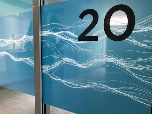
Stefanie Posavec created art at the Papworth Hospital, which was an Inpatients Ward. She was commissioned to create artwork that considered the human body and was human-scaled. Most importantly, she wanted it to be calming to patients who had just come out of surgery. I admire her work as she chose to show important computational information through understanding of the heartbeat, breath and lungs, and the blood and blood vessels that connect the two. Then, by incorporating “calming” nature she focused on aesthetics which showed waveforms (which is shown in ocean waves and heartbeats), branching (which is shown in the lungs and trees) etc. This ended up fulfilling the needs of both the patients and the staff as if offered patient privacy as well as a clear line – of-sight for nurses and staff. It was also really cool how she mapped data to concept showing how “medical data relevant to either the heart, lungs, or blood” was used as a ‘seed’ for that floor’s specific artwork.
Project-07: Composition with Curves
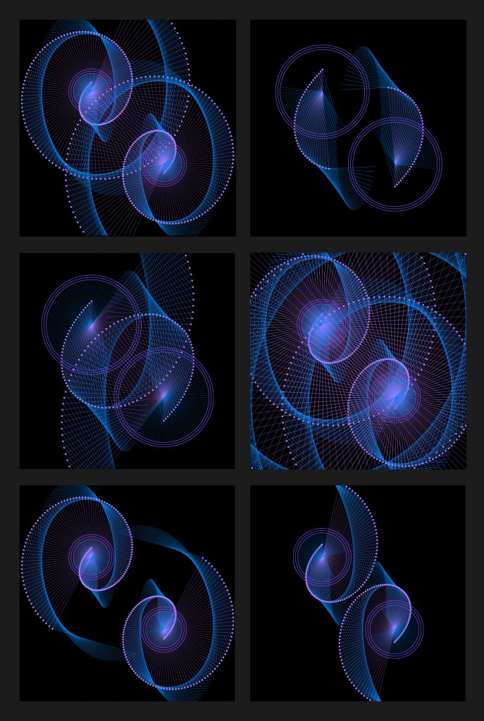
Reference Curve: Atzema Spiral
Move the mouse up and down to change the rotation angle
Move the mouse left and right to change the radius
//Xinyi Du
//15104 Section B
//xinyidu@andrew.cmu.edu
//Project-07

//Referrence Curve: Atzema Spiral
//move the mouse up and down to change the rotation angle
//move the mouse left and right to change radius

function setup() {
    createCanvas(480, 480);
    background(250);
}

function draw() {
    background(0);
    //draw the pair of lines that change with mouseX and mouseY
    lines1(mouseX, mouseY);
    lines2(mouseX, mouseY);
}

//define the function to draw the lines
function lines1 (R, A) {
    //constrain the angle and radius and map them to specific ranges
    RR = constrain(R, 0, width);
    AA = constrain(A, 0, height);
    //radius with the range(20, 20)
    r = map(RR, 0, width, 20, 50);
    //angle within the range(50, 800)
    a = map(AA, 0, height, 50, 800);

    //for loop to draw the lines and circles
    for (angle = 57.2957795; angle < 57.2957795+a; angle += 3) {
        push(); //push to save the orgin tranformation

        //translate the origin to (width/3, width/3)
        translate(width/3, width/3);
        //polar coordinates according to Atzema Spiral
        var t = radians(angle);
        var x = x3+ r * ( sin(t)/t - 2*cos(t) - t*sin(t) );
        var y = y3+ r * ( -cos(t)/t - 2*sin(t) - t*cos(t) );
        //another series of polar coordinates with 60 more degrees of angle
        var t2 = radians(angle+60);
        var x2 = x3 + (r) * ( sin(t2)/t2 - 2*cos(t2) - t2*sin(t2) );
        var y2 = y3 + (r) * ( -cos(t2)/t2 - 2*sin(t2) - t2*cos(t2) );
        //reference circle polar coordinates
        var radius = 2*r; //radius of the circle
        var x3 = radius * cos(radians(angle));
        var y3 = radius * sin(radians(angle));

        strokeWeight(0.5);
        //purple and opacity 90 of the lines from center to polar coordinates
        stroke(183, 125, 255, 90);
        line(0, 0, x, y);

        //blurish purple
        stroke(104, 81, 225);
        noFill();

        //three circles
        ellipse(0, 0, radius*2, radius*2);
        ellipse(0, 0, radius*2+10, radius*2+10);
        ellipse(0, 0, radius*2+20, radius*2+20);

        //blue
        stroke(1, 124, 228);
        //lines from first series of polar coordinates to the second series
        line(x, y, x2, y2);
        //lines from center to the reference circle
        line(0, 0, x3, y3);

        //purple
        stroke(183, 125, 255)
        fill(183, 125, 255);
        //small circles
        circle(x, y, 3);

        pop(); //pop to return to the original setting of the origin
    }

}

//rotate 180 degrees of the lines1
function lines2 (R, A) {
    //tranlate the origin
    translate(width, height);
    rotate(radians(180));
    //call the function lines1
    lines1(R, A);
}
Looking Outwards 07: Information Visualization
Flight Patterns
http://www.aaronkoblin.com/work/flightpatterns/index.html
Aaron Koblin, Scott Hessels, and Gabriel Dunne
Celestial Mechanics–Flight Patterns
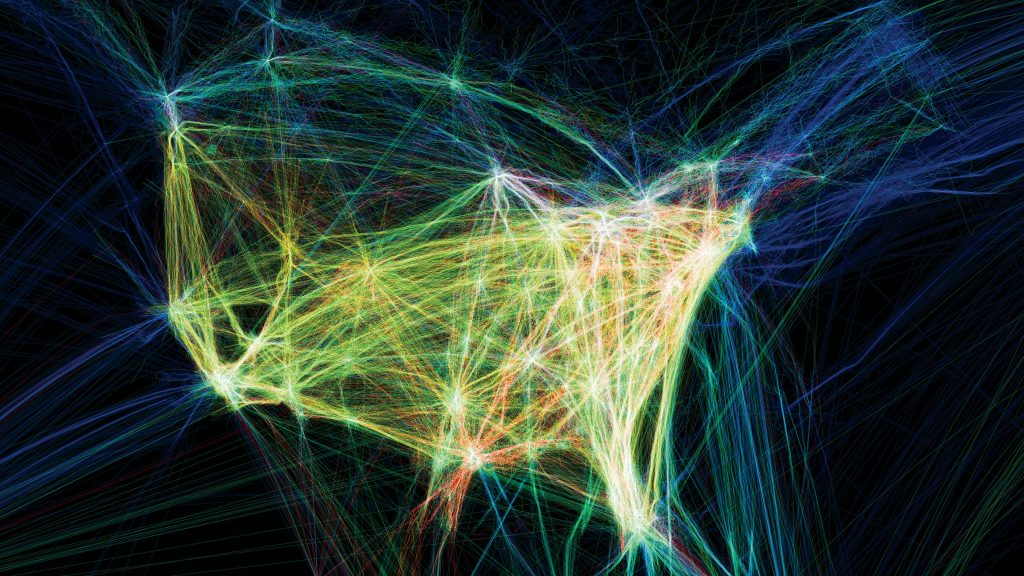
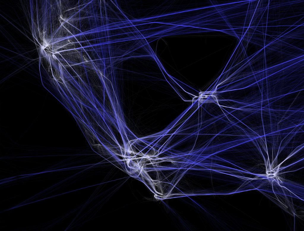
The Project is an exploration and visual representation of flight patterns in North America.
What I admire a lot about the project is that the project not only provides status images to show the overall patterns and frequency of flights in different cities but also a video to show the dynamic routes of the flights.
The data used is from Federal Aviation Administration and the Processing programming environment and Adobe After Effects and/or Maya are applied for the visualization and representation of data.
The background is set in black and the flights are set in lighter colors, and the denser the lines or the more frequent the flight routes, the brighter the colors and closer the colors to white. This use of contrast of dark background and light lines creates strong contrast and makes the flights more prominent. It is also easy to identify the places where flights are more frequent by comparing the line weights and colors. On the aesthetic aspect, the overall effects of both the diagrams and the video are very visually appealing and the lines remind the audience of lightning or fireworks.
Looking Outwards-07
For this week’s blog post about information visualization, I picked the work by Moritz Stefaner “The Rhythm of Food”. It is a project that analyzes different food seasonality. He gathers the information we learn about food culture by looking at Google search data. The project collaborates with Google News Lab, and sheds light on the many facets of food seasonality, based on twelve years of Google search data. In order to investigate seasonal patterns in food searches, the team developed a new type of radial “year clock” chart to reveal seasonal trends for food items. The way it works is each segment of the chart indicates the search interest in one of the weeks of the past 12 years, with its distance from the center showing the relative search interest, and the color indicating the year. I admire the way Stefaner turns a huge amount of data into an easily visualizable graph. It was interesting to see how cultural and social influence has on the data result.
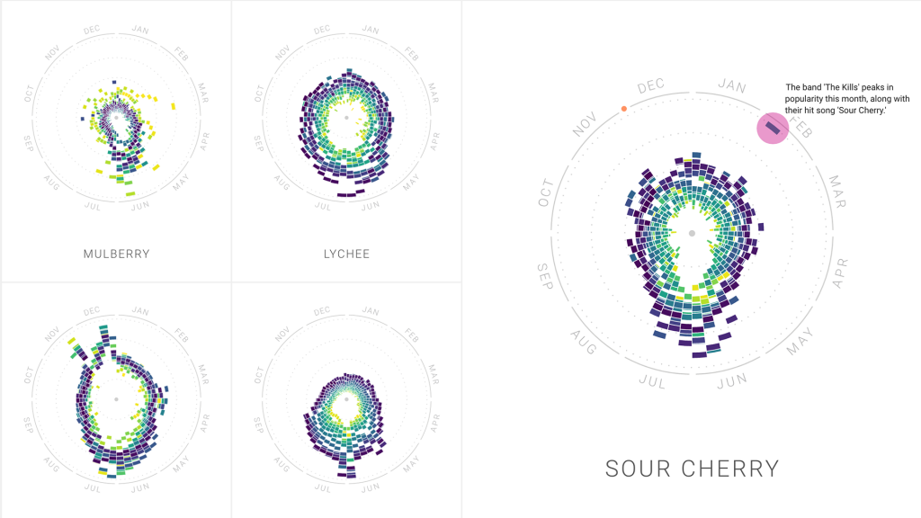
Creative direction, data visualization, design: Moritz Stefaner
Design and development: Yuri Vishnevsky
Illustration: Stefanie Weigele
Project-07-curves
The most difficult part of this project is to find out how which curve formula to use for my design. I played around with different colors and shape overlapping and I like the flower shape it makes.
//Jenny Wang
//sectionB
//jiayiw3@andrew.cmu.edu
//project - 07 - curves

var nPoints = 150;

function setup() {
    createCanvas(480, 480);
    background(29,7,79);//dark purple
    frameRate(10);
}

function draw() {
    push();
    //make the center of canvas the origin
    translate(width/2,height/2);

    //draw loop for the curves 1 & 2
    background(29,7,79);//dark purple
    curve1();
    curve2();
    curve3();
    pop();
}

function curve1(){

    //Epicycloid Involute
    //https://mathworld.wolfram.com/EpicycloidInvolute.html

    //set varibale
    var x;
    var y;
    var a = mouseX/8
    var b = mouseY/8

    beginShape();
    noFill();
    stroke(247,246,208);//light yellow
    for(var i=0; i<nPoints; i++){
            var t = map(i,0,nPoints,0,TWO_PI);
            x = (a+b)*cos(t)-b*cos(((a+b)/b)*t);
            y = (a+b)*sin(t)-b*sin(((a+b)/b)*t);
            vertex(x,y);

        endShape(CLOSE);
    }
}

function curve2(){

    //Epicycloid Involute
    //https://mathworld.wolfram.com/EpicycloidInvolute.html

    //set variable
    var x;
    var y;
    var a = mouseX/5
    var b = mouseY/5

    beginShape();
    noFill();
    stroke("white");//white
    for(var i=0; i<nPoints; i++){
            var t = map(i,0,nPoints,0,PI+QUARTER_PI);
            x = (a+b)*cos(t)-b*cos(((a+b)/b)*t);
            y = (a+b)*sin(t)-b*sin(((a+b)/b)*t);
            vertex(x,y);

        endShape(CLOSE);
    }
}

function curve3(){

    //Epicycloid Involute
    //https://mathworld.wolfram.com/EpicycloidInvolute.html

    //set variable
    var x;
    var y;
    var a = mouseX/3
    var b = mouseY/3

    beginShape();
    noFill();
    stroke("pink");//pink
    for(var i=0; i<nPoints; i++){
            var t = map(i,0,nPoints,0,PI);
            x = (a+b)*cos(t)-b*cos(((a+b)/b)*t);
            y = (a+b)*sin(t)-b*sin(((a+b)/b)*t);
            vertex(x,y);

        endShape(CLOSE);
    }
}Project 07 – srauch – curves
Here is my program that runs on curves. I call it “laser ballerinas”. Move your mouse left to right to increase the size of the curves and the overall rotation, and move your mouse up and down to change the number of “lobes” on each curve. Click to change the colors of each lobe!
//Sam Rauch, section B, srauch@andrew.cmu.edu, project 07
//This code produces a "laser ballerinas" using epicycloid curves. Ten epicycloid curves of decreasing
//size and random colors are drawn on top of each other to produce "nested curves", and six nested curves
//are drawn in a hexagon pattern around the center of the canvas, which spins. MouseX controls the size of
//the curves and the rotation of the hexagon pattern, while mouseY controls the number of "lobes" produced
//in each epicycloid curve. Click to change the colors of the ballerinas!

var coloroptions;

function setup() {
    createCanvas(400, 400);
    background(220);
    text("p5.js vers 0.9.0 test.", 10, 15);

    coloroptions = [];
    for (var i = 0; i < 9; i++) {
        coloroptions[i] = color(random(255), random(255), random(255));
    }

}

function draw() {
    background(0);
    translate(width/2, height/2);

    //create spin the hexagon of curves around the center of the canvas according to mouseX
    push();
    var spinamt = map(mouseX, 0, width, 0, 2*PI)
    rotate(spinamt);


    //draws six nested curves in a hexagon pattern
    for (var i = 0; i < 6; i++){
        push();
        translate(100, 0);
        nestedCurve();
        pop();
        rotate(radians(60));
    }

    pop();

}

//generates epicycloid curve (https://mathworld.wolfram.com/Epicycloid.html) with center at 0,0
function drawCurve(color){

    noFill();
    stroke(color);
    strokeCap(ROUND);
    strokeJoin(ROUND);
    strokeWeight(3);

    var points = 80;
    var xValues = [];
    var yValues = [];
    var a = mouseX/4; //radius of larger inner circle
    var b = constrain(mouseY/10, 0, a) ; //40; //radius of smaller outer circle
    var theta = 0;

    //generating x and y values based on epicycloid curve forumla, and increasing the center angle
    //by a small amount
    for (var i = 0; i < points; i++) {
        theta += radians(5);
        xValues[i] = (a+b)*cos(theta) - b*cos(((a+b)/b)*theta);
        yValues[i] = (a+b)*sin(theta) - b*sin(((a+b)/b)*theta);
    }

    //plotting x and y values
    beginShape();
    for (var i = 0; i <points; i++) {
        vertex(xValues[i], yValues[i]);
    }
    endShape();
}

//draws ten epicycloid curves of random colors nested inside each other
function nestedCurve() {
    push();

    var size = 1;
    var sizeIncrement = 0.1;

    //draws ten epicycloid curves, but for each one, decreases scale and change color
    for (var i = 0; i < 9; i++) {
        scale(size);

        var col = coloroptions[i];
        drawCurve(col);
        size -= sizeIncrement;
    }

    pop();
}

function mousePressed(){
    for (var i = 0; i < 9; i++) {
        coloroptions[i] = color(random(255), random(255), random(255));
    }
}![[OLD SEMESTER] 15-104 • Introduction to Computing for Creative Practice](../../../../wp-content/uploads/2023/09/stop-banner.png)