Project 07: Composition with Curves

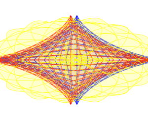
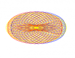
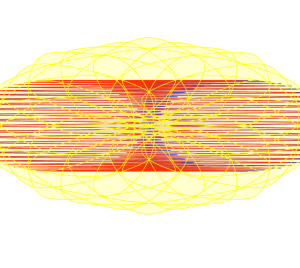
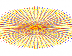
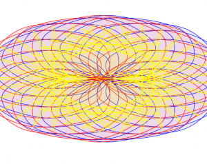
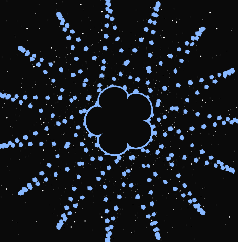
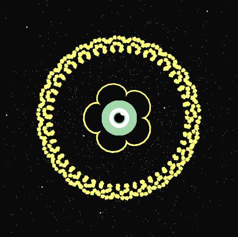
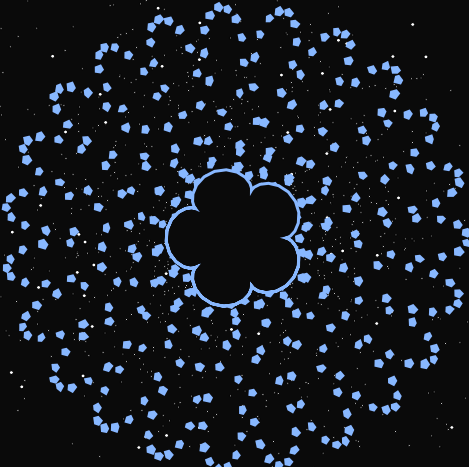
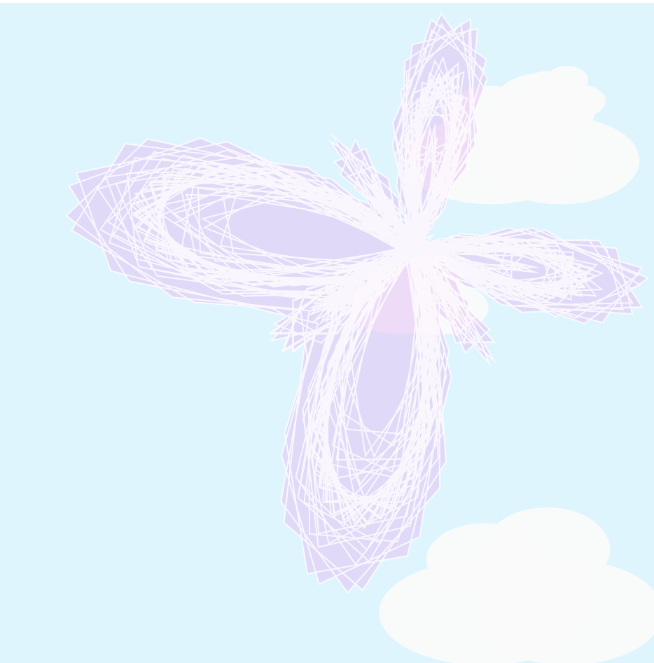
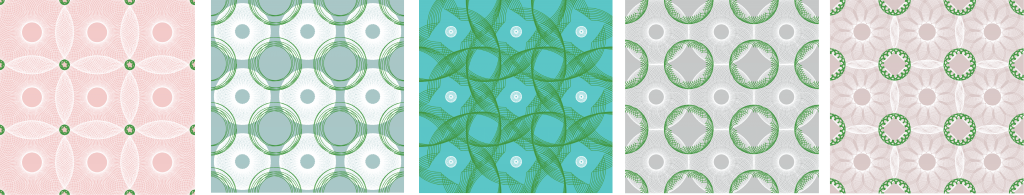
I used a series of three hypocycloid curves (based on the hypocycloid pedal formula) to model an interactive color wheel. I wanted to juxtapose the complex curves and forms with the simplicity of primary colors.

colorwheel
var nPoints = 100	//number of points in each curve

function setup() {
    createCanvas(480, 480);
}

function draw() {
	var halfWide = width/2
	var halfTall = height/2
	background('white')
	push();
	translate(halfWide+10, halfTall)	//move center of curves to center of canvas, offset by 10 tp create overlap later
	HypocycloidBlueCurve()	//draw blue curve
	pop();
	translate(halfWide-10, halfTall);	//move center of curves to center of canvas but offset the other way so overlaps with blue
	HypocycloidCurve()	//draw red curve
	translate(5, 0)	//move back to true canvas center to draw yellow curve over both red and blue
	HypocycloidYellowCurve()	//draw yellow curve
}

function HypocycloidCurve(){
    var a1 = constrain(mouseY, 0, 300, 150, 180); //size changes as vertical mouse position changes
    var b1 = 45;
    var n1 = int(mouseY / 6)	//number of cusps of the curve varies with vertical mouse position

    stroke('red');	//change stroke color to red
    strokeWeight(1);
    fill(255, 0, 0, 20);	//change fill to transparent red

    //create curve, using https://mathworld.wolfram.com/HypocycloidPedalCurve.html base formula for Hypocycloid Pedal Curve
    //map points of curve to circle
    beginShape();
    for (var i = 0; i < nPoints; i++) {
        var theta = map(i, 0, nPoints, 0, TWO_PI);     
        var x1 = a1*(((n1-2)*(cos(theta)-cos((1-n1)*theta)))/(2*n1))
        var y1 = a1*(((n1-2)*(cos(theta*(1-0.5*n1))*sin(0.5*n1*theta)))/(2*n1))
        curveVertex(x1, y1);
    }
    endShape(CLOSE); 
}

//draw blue hypocycloid, same as red but in blue
function HypocycloidBlueCurve(){
    var a1 = constrain(mouseY, 0, 300, 150, 180); //size changes as vertical mouse position changes
    var b1 = 45;
    var n1 = int(mouseY / 6)	//number of cusps of the curve varies with vertical mouse position
    fill(0, 0, 255, 20)	//fill transparent blye
    stroke('blue');	//set stroke color to blue
    strokeWeight(1);
    //create curve, using https://mathworld.wolfram.com/HypocycloidPedalCurve.html base formula for Hypocycloid Pedal Curve
    //map points of curve to circle
    beginShape();
    for (var i = 0; i < nPoints; i++) {
        var theta = map(i, 0, nPoints, 0, TWO_PI);     
        var x1 = a1*(((n1-2)*(cos(theta)-cos((1-n1)*theta)))/(2*n1))
        var y1 = a1*(((n1-2)*(cos(theta*(1-0.5*n1))*sin(0.5*n1*theta)))/(2*n1))
        curveVertex(x1, y1);
    }
    endShape(CLOSE); 
}
//draw yellow hypocycloid
function HypocycloidYellowCurve(){
    var a1 = constrain(mouseY, 0, 300, 150, 180); //size changes as vertical mouse position changes
    var b1 = 45;
    var n1 = int(mouseY / 10)	//number of cusps of the curve varies with vertical mouse position
    fill(255, 255, 0, 50)	//set fill color to a transparent yellow
    stroke('yellow');	//set stroke color to yellow
    strokeWeight(1);
	//create curve, using https://mathworld.wolfram.com/HypocycloidPedalCurve.html base formula for Hypocycloid Pedal Curve
    //map points of curve to circle
    beginShape();
    for (var i = 0; i < nPoints; i++) {
        var theta = map(i, 0, nPoints, 0, TWO_PI);     
        var x1 = a1*(((n1-2)*(cos(theta)-cos((1-n1)*theta)))/(2*n1))
        var y1 = a1*(((n1-2)*(cos(theta*(1-0.5*n1))*sin(0.5*n1*theta)))/(2*n1))
        curveVertex(x1, y1);
    }
    endShape(CLOSE); 
}

Looking Outwards – 07

Ben Fry’s piece called All Streets was created on April 24, 2008. It is compilation of 240 million segments of road compressed into the shape of the United States continent. Ben was joined by three teammates – Katy assembled high-resolution images for offset printing, James made sure that the prints’ densities were appropriate for the piece, and Chris helped write software. This software created tiles that could be combined into a high-quality, HD image.

All Streets by Ben Fry (April 24, 2008)

I admire this aspect of the project because compiling such an enormous amount of images into one is a feat, considering that most software has a hard time dealing with images more than 30,000 pixels wide. The software program that he developed is called Processing, an open source programming environment that allows for computational design and interactive media. His artistic sensibility in processing and visualizing data is clearly manifested in the final form of this piece. His interactions with informational data is transformed into piece that takes millions of individual road segments into one unified artwork.

A closer look at All Streets – roadless terrain creates the topography of the Appalachian Mountains

LO – 07 – Information Visualization

Fernanda Viegas, Wind Map, 2012. 

Fernanda Viegas’ “Wind Map”.

This project creates a real-time, or a “living portrait”, wind map of the United States during the winter months and uses the data to visualize an art piece in the process. The project uses motion of white lines over a black map of the U.S. to show the wind motions and heaviness by layering the white wind lines. 

Viegas notes that while it was an artistic endeavor originally, the map provides a variety of functions where people have used it for bird migration patterns, bicyclists, etc. Viegas uses data for this project from the National Digital Forecast Database and combines it with computational circulations that project the data in an abstracted, artistic way. The Wind Map uses “comet-like trails” to show the motion of the wind lines. The map is made entirely in HTML and JavaScript. 

Hurricane Sandy, October 30 Wind Map.

This project is successful in its multi-purpose presentation of wind data in the U.S. and its additional artistic purpose. Computationally creating the Wind Map creates a direct way to have updates to the data sets as the wind directions, intensity, etc. changes from day to day. This conveys accurate data for the day but also creates an art piece that is mesmerizing because of its constant movement. The Wind Map additionally impressively communicates the forecast data in a simplistic and easy to understand map consisting of two main elements; the base map and the wind lines.

Project – 07 – Curves

sketch
/* 
 * Amy Lee 
 * amyl2
 * Section B 
 */ 

// Array variables for star X and Y positioning 
var starX = []; 
var starY = []; 
var r = 5; 
var r2 = 10; 
var nPoints = 5; 
var nPoints2 = 10; 
var separation = 120; 

function setup() {
    createCanvas(480,480);
    // Random placement of stars
    for (i = 0; i < 60; i++){
    	starX[i] = random(10,470); 
    	starY[i] = random(10,470); 
    }
    frameRate(7); 
}

function draw() {
	background(10); 

	// Time variable for stars 
	var s = second(); 

	// Setting randomGaussian ellipses in the background 
    push(); 
    translate(width/2,height/2); 
    for (var i = 0; i < 1000; i++){
    	fill(255); 
    	ellipse(randomGaussian(0,120),randomGaussian(0,120),2.2,2.2);
    }
    pop(); 

    // New star every second
    for( i = 0; i < s; i++){
    	fill(255); 
    	ellipse(starX[i],starY[i],4,4); 
    }

	// Calling on Hypotrochoid Function
    push(); 
    noStroke(); 
    translate(width/2,height/2); 
    drawHypotrochoid(); 
    pop();

    // Calling on Ranuculus Function
	drawRanuculus();

	// Drawing hidden alien, only appears when mouse distance from center is < 50
	push(); 
	for(var y = 200; y < 280; y += 5){
		for (var x = 200; x < 280; x += 5){
			noStroke(); 
			fill(173,212,173); 
			if(nearMouse(x,y) == true){
				// Face
				ellipse(241,240,70,70); 
				// Eye 
				fill(255); 
				ellipse(241,240,40,40); 
				// To make eye follow mouseX when mouseX is near 				
				fill(173,212,173); // green iris
				if (mouseX < 256 & mouseX > 230){ 
					ellipse(mouseX,240,25,25);
				} else {
					ellipse(241,240,25,25); 
				}
				// Pupil 				
				fill(0) 
				if (mouseX < 256 & mouseX > 230){ 
					ellipse(mouseX,240,20,20);
				} else {
					ellipse(241,240,20,20); 
				}				
				fill(255); 
				ellipse(248,230,10,10); 
			}
		}
	}
	pop(); 
} 


function drawHypotrochoid() {
	// Setting Hypotrocoid Variables
	for (var t = 0; t < 360; t++){
  		var h = map(mouseY, 0, height/4, height/2, height/4);
    	var a = 150;
    	var b = map(mouseY,0,height/2,1,2);

	var x = (((a-b)*cos(radians(t))) + h*cos(((a-b)/b)*radians(t))); 
	var y = (((a-b)*sin(radians(t))) - h*sin(((a-b)/b)*radians(t)));

	// Draw pentagons 
    beginShape();
    for (var i = 0; i < nPoints; i++) {
    	noStroke(); 
    	// Pentagons change color as mouseY changes 
		if (mouseY <= 80){
			fill(255,142,157); //Red 
		} else if (mouseY > 80 & mouseY <= 160){
			fill(255,210,142); // Orange 	
		} else if (mouseY > 160 & mouseY <= 240){
			fill(255,252,142); // Yellow 	
		} else if (mouseY > 240 & mouseY <= 320){
			fill(192,255,142); // Green 
		} else if (mouseY > 320 & mouseY <= 400){
			fill(142,188,255); // Blue 	
		} else if (mouseY > 400 & mouseY <= 480){
			fill(157,142,255); // Purple	
		} else {
			fill(random(255),random(255),random(255)); 
		}	
		// Setting variables for pentagons
        var theta = map(i, 0, nPoints, 0, TWO_PI);
        var px = r * cos(theta);
        var py = r * sin(theta);
        // Draw pentagon shape with random jitter 
        vertex(x+px + random(-1, 1), y+py + random(-1, 1));
   	}
    endShape(CLOSE);
	}
}

function drawRanuculus() {
	push(); 
	translate(2 * separation, height/2);
	// Setting stroke colors according to how mouseY changes 
		if (mouseY <= 80){
			stroke(255,142,157); //Red 
		} else if (mouseY > 80 & mouseY <= 160){
			stroke(255,210,142); // Orange 	
		} else if (mouseY > 160 & mouseY <= 240){
			stroke(255,252,142); // Yellow 	
		} else if (mouseY > 240 & mouseY <= 320){
			stroke(192,255,142); // Green 
		} else if (mouseY > 320 & mouseY <= 400){
			stroke(142,188,255); // Blue 	
		} else if (mouseY > 400 & mouseY <= 480){
			stroke(157,142,255); // Purple	
		} else {
			stroke(random(255),random(255),random(255)); 
		}	
	strokeWeight(3); 
	fill(10); 
	beginShape();
    for (var i = 0; i < nPoints2; i += 0.1){
      var px2 = r2 * (6 * cos(i) - cos(6 * i));
      var py2 = r2 * (6 * sin(i) - sin(6 * i));
      vertex(px2, py2);
    }
    endShape();
    pop()
}

function nearMouse(x,y){
	if(dist(x,y,mouseX,mouseY) < 50){
		return true;
	} else {
		return false; 
	}
}


For this project, I played around with the Hypotrochoid and Ranuculus curves to create these designs. I wanted to give this an outer space feel, so I also added a Gaussian distribution of ellipses to resemble stars in the background. When the distance of the mouse is close to the center, an alien eye is revealed. The colors of the curves according to the mouseY position and an additional larger star is added every second. It definitely has a chaotic look to it but I thought that it fit the theme since space is far from organized.

Project-07-Curves

This is based on a hypotrochoid, which is a point rotating around a circle that is rotating around a larger circle. The point is supposed to create a looping pattern around the larger circle. I changed this by having the position of the mouse affect how fast the point would rotate, breaking the looping pattern created by a hypotrochoid. In addition, I also had the mouse affect the speed at which the inner circle was rotating around the outer circle and the distance the point is from the inner circle. It is a little activity where you can try to fill in the backgroudn with the blue but it is challenging because the point in always rotating and affected by the mouse position.

sketch

var r = 0 // rotation angle of outer circle
var r1 = 0 // rotation angle for inner circle
function setup() {
    createCanvas(480, 480);
    background(0);
    strokeWeight(0);
}

function draw() {
    fill(255);
    textSize(20);
    text('Fill in the background!',0,20);
    translate(width/2,height/2);
    scale(.8);
    speedr = map(mouseX,0,480,0,3,true);
    rotate(radians(r));
    r += speedr
    outercircle();
    innercircle();

    function innercircle(){
      push();
      fill(0,255,0);
      translate(0,170);
      speedr1 = map(mouseY,0,480,1,5,true);
      rotate(radians(r1));
      r1 += speedr1
      circle(0,0,60);
      point();
      pop();

      function point(){
        fill(0,0,255);
        cdistance = map(mouseX,0,480,20,150);
        circle(0,cdistance,30);
      }
    }
    function outercircle(){
      fill(255,0,0);
      circle(0,0,400);
    }
}

Looking Outwards-07

Nathan Yau is using data from the running app RunKeeper to create visualizations of the most taken courses or paths runners take in different cities. Nathan is a statistician from FlowingData who focuses on information design, as seen in the informational maps he has created below. He finds that visualization is a key way to make data more accessible and attractive. 

He created these data visualizations for 18 major US cities, including Chicago, LA, and New York City. He simply concluded that most runners love to run near nature, which are near water and parks.

To create these visualizations he may have used photoshop to collage all the paths of every runner or maybe if he used p5js he created arrays that marked each location as a point and when each location is marked the density increases, which increases the deepness of the purple as well.

Philadelphia running paths
New York City running paths

Project 07: Composition with Curves

I decided to go with a butterfly curve because I thought it looked cool. Because of the name, I decided to make my project a butterfly flying in the sky. For the background, I just reused my clouds that I made for last week’s deliverables. Instead of having them move depending on what minute it was, I just set a constant to add to the x values of the ellipses the clouds were made of.

butterflyDownload
var translateX;
var translateY;
var nPoints=1000;
var butterfly=true;
var cloudScale=[0.5, 0.75, 1, 1.25, 1.5];
var x=0;
var dx=0.1;

function setup() {
    createCanvas(480, 480);
    translateX=width/2;
    translateY=height/2;
}

function draw() {
    background(222, 245, 253);
    drawClouds();
    push();
    translate(translateX, translateY);
    drawButterfly();
    pop();
}

function drawButterfly(){
    //Butterfly curve https://mathworld.wolfram.com/ButterflyCurve.html
    //this draws a butterfly curve to make the butterfly
    beginShape();
    scale(50);
    strokeWeight(0.02);
    stroke(255, 200);
    var x;
    var y;
    var angle=radians(map(mouseY, 0, height, 0, 360)); //rotation depends on mouseY
    rotate(angle);
    var m=map(mouseX, 0, width, 0, 25); //the size/extent of the curve of the butterfly depends on mouseX
    for (var i=0; i<nPoints; i++){
        var t=map(i, 0, nPoints, 0, m*TWO_PI); //var m is multiplied times the upper limit of the map function
        x=sin(t)*(exp(cos(t))-2*cos(4*t)+pow(sin((1/12)*t), 5));
        y=cos(t)*(exp(cos(t))-2*cos(4*t)+pow(sin((1/12)*t), 5));
        vertex(x, y);
        fill(228, 198, 245, 150);
    }
    endShape();
}

function mousePressed(){
    //changes position depending on where you click
    translateX=mouseX;
    translateY=mouseY;
}

function drawClouds(){
    //smallest cloud--cloud 1
    push();
    fill(250, 250);
    noStroke();
    scale(cloudScale[0]);
    translate(500,100);
    cloud();
    pop();

    //cloud 2
    push();
    fill(250, 250);
    noStroke();
    scale(cloudScale[1]);
    translate(100, 250);
    cloud();
    pop();

    //cloud 3
    push();
    fill(250, 250);
    noStroke();
    scale(cloudScale[2]);
    translate(400, 350);
    cloud();
    pop();

    //cloud 4
    push();
    fill(250, 250);
    noStroke();
    scale(cloudScale[3]);
    translate(0, 50);
    cloud();
    pop();

    //cloud 5
    push();
    fill(250, 250);
    noStroke();
    scale(cloudScale[4]);
    translate(-50, 250);
    cloud();
    pop();
}

function cloud(){
    ellipse(x+30, 10, 60, 40);
    ellipse(x+40, 40, 90, 50);
    ellipse(x, 40, 100, 50);
    ellipse(x, 15, 55, 35);
    x=x+dx;
    //once the clouds go off the screen, they reappear on the other side
    if(x>width){
        x=0;
    }
}

It rotates depending on where mouseY is and also draws the curve as mouseX goes from left to right.

You can also click to change the origin of the image and move the butterfly around.

Looking Outwards 07: Information Visualization

This week, I decided to look at Chris Harrison’s Amazon Book Map He looked at 735,323 books and captured similarity data between them based on what Amazon recommended. He then color coded them depending on genre and created a visualization of his findings. I really admire the effort he put into it and the way it all came together in a mosaic like pattern. The algorithms he used created the layout and clustering but he noted that his algorithm didn’t work well for unstructured graphs. Harrison has created a lot of these visualizations and is trying to look at a new way to display data, and I think he was very successful with this. Especially color coding, it allows the user to see how different genres mesh together in a more user-friendly way.

Chris Harrison, Amazon Book Map

LO-7: Unnumbered Sparks, Janet Echelman, 2014

I was attracted to this work at the first sight. It is a monumental, beautiful sculpture work flowing in the sky, consisted of an intricate, color-changing net. The audience can interact with the piece by connecting to the project’s wifi and give instructions to the website promoted, such as changing colors, moving parts around, etc. I like how it gives the audience the chance to be the creators of this art work and fully participate in it by taking out the artist’s role as the maker. I also like the sense of vulnerability and mobility in this work. The piece is like a floating, colorful, and constantly changing nebula that has fragile, mysterious, mobile beauty.

The team collaborated with Janet Echelman, a sculpture artist who works with public space. What they used to build this sculpture is a kind of fiber that is fifteen times stronger than steel. And the sculpture was put up into the middle of an active city’s sky. The project team built the modal in Chrome with webGL. They then modified parameters to get the complex behaviors they were looking for. The mobile and interactive aspect of the piece was made possible by a language developed by the team. It sits in between Javascript and C language. People’s input would then directly influence what they see. The team commented on this, saying “they can draw and paint with light,…people are the Co-creators. Seeing the delight and wonder on people’s faces is the best reward for the team.”

Project-07 Curves

curves
var r = 0;    //red color variable 

var a = 0;    //radius of circle a (inner circle) for parametric function 
var b = 0;    //radius of circle b (fixed circle) for parametric function  
var h = 0;    //distance from center of inner circle

var theta = 0;    //angle variable
 
function setup() {
    createCanvas(480, 480); 
    background(220);
}

function draw() {

	//changing red level of background  
	r = map(mouseX, 0, 480, 0, 255); 
    background(r, 200, 200);

    //creates 9 Hypotrochoid curves
    for (var x = 0; x <= 400; x += 160) {
        for (var y = 0; y <= 400; y += 160) {
            push();
            translate(x+80, y+80);
            drawHypotrochoid();
            pop();
        }
    }

    //creates 16 Hypotrochoid Evolute curves
    for (var x = 0; x <= 480; x += 160) {
        for (var y = 0; y <= 480; y += 160) {
            push();
            translate(x, y);
            drawEvolute();
            pop();
        }
    }
}

function drawHypotrochoid() {

    //curve based on the Hypotrochoid equation 

    strokeWeight(0.5);
    stroke(255);
    noFill();
    beginShape();    

    a = map(mouseX, 0, 480, 1, 70);
    b = map(mouseY, 0, 480, 1, 5);
    h = map(mouseX, 0, 480, 1, 40);

        for (var i = 0; i < 2000; i++) {

            var x = (a-b)*cos(theta) + h*cos((a-b)/b*theta);
            var y = (a-b)*sin(theta) + h*sin((a-b)/b*theta);
            var theta = map(i, 0, 360, 0, TWO_PI);
        
            vertex(x, y);
        }  

    endShape();

    pop();
}

function drawEvolute() {

    //curve based on the Hypotrochoid Evolute equation
    
    strokeWeight(1);    
    stroke(0, 150, 0);

    noFill();
    beginShape();    

    a = 8*map(480-mouseX, 0, 480, 1, 30);
    b = 2*map(480-mouseY, 0, 480, 1, 20);
    h = 3*map(480-mouseX, 0, 480, 1, 10);

        for (var i = 0; i < 4000; i++) {

            var x = (a-b)*cos(theta) + h*cos((a-b)/b*theta);
            var y = (a-b)*sin(theta) + h*sin((a-b)/b*theta);
            var theta = map(i, 0, 480, 0, TWO_PI);
        
            vertex(x, y);
        }  

    endShape();

    pop();
}
screenshots of cursor at different points

For this project, I tried out a few of the equations from the reference and liked the look of the Hypotrochoid the best. Once I had the Hypotrochoid curve working I want to add some visual interest by replicating them with a loop. Once that was done, I added another curve, the Hypotrochoid Evolute and replicated that with a loop too. After the curves were all in place, I added the changing background. The biggest challenge was understanding how changing the values of variables in the equations effected the curve but once I was able to get that it was fun to mess around with!