LookingOutwards-07

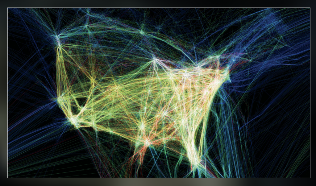
Flight Patterns by Aaron Koblin.

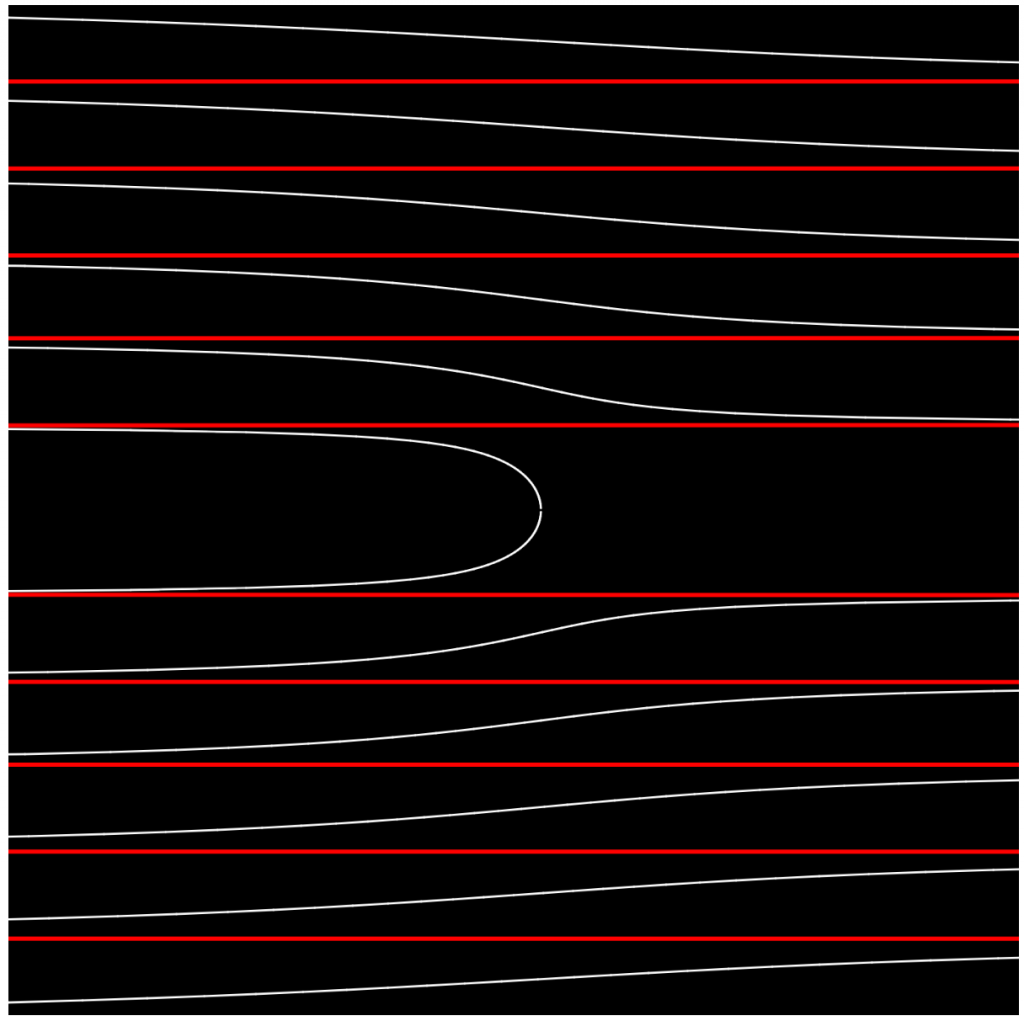
For this week’s Looking Outwards on the topic of informational visualization, I decided to look at the works by Aaron Koblin, and in particular, I was drawn to his Flight Patterns visualization (http://www.aaronkoblin.com/project/flight-patterns/). In this project, he took many data values and mapped out the paths of air traffic across North America. The visualization is abstracted to show strings of moving, glowing lines showing the progression and density of flight routes. When there is high air traffic and many routes intersect, the lines seem to glow at the intersection point. When the supposed “planes” travel away from each other, the movement fades out. To make this computational visualization, Koblin worked with his colleagues and plotted the data using the Processing programming environment. For the algorithms themselves, I think there is a component of controlling the amount of brightness of the lines. When they come in close proximity, they glow brighter, and this effect would have been created using conditionals and loop statements. I think the artist was able to take the shape of North America and make that appear obvious in the final product through creating color boundaries that show the distinction between “land” and “sea” spaces. I find this work really interesting, and it reminded me of a similar map that I was shown in my global history class, which mapped out the traffic patterns of slave ships to America over time.

Project 07- Curves

sketchDownload

//Shruti Prasanth
//Section C
//Project 07 Curves


var numPoints = 400;
function setup() {
    createCanvas(480, 480);
}


function draw() {
    background(105,179,183); //BLUE background
    
    for (var x = 80; x <= 460; x += 80) {   //number of elements in the grid
        for (var y = 80; y <= 460; y += 80) {
            push();
            translate(x, y);
            HypocycloidPedal();
            pop();
        }
    }

}

function HypocycloidPedal() {
    //radius
    var a = map(mouseX, 0, 480, 0, 120); 
    var b = map(mouseX, 0, 480, 0, 120);

    strokeWeight(mouseY/50, mouseX/50); //change in stroke thickness
    stroke(255); //WHITE 
    noFill();

  
    beginShape();
    for (var i=0; i<numPoints; i++) {
        var angle = map(i, 0, 100, 0, TWO_PI);
        var n = 8; //number of petals

        x = a * (((n-1) * cos(angle)) + (cos((n-1) * angle)) );
        y = a * (((n-1) * sin(angle)) - (sin((n-1) * angle)) );

        vertex(x, y);       
    }
    endShape();     
}


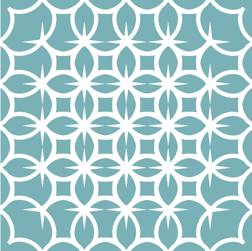
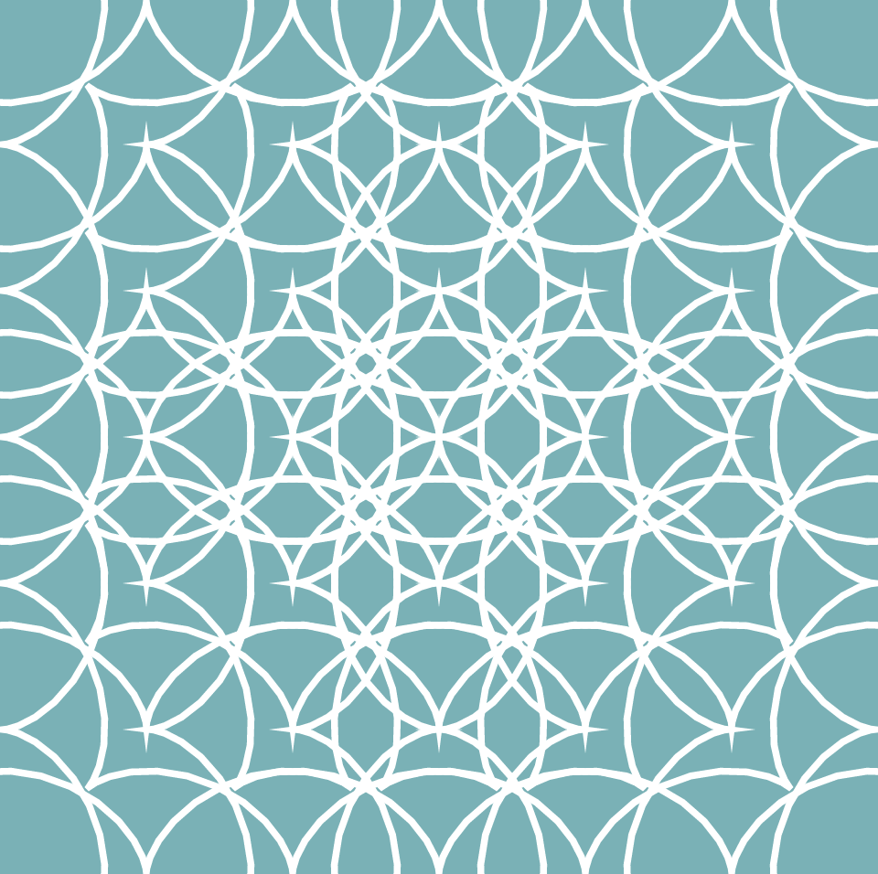
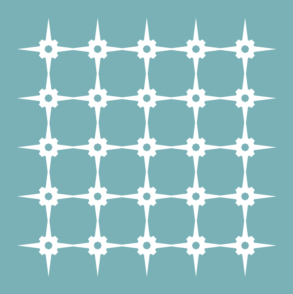
For my project I was inspired by ornate printed patterns and mosaics. I wanted to make something that formed interesting shapes when the curves intersected and dynamically changed. Here are some of the screenshots of the different patterns that are created when you move your mouse around the canvas:

Looking Outwards 07: Information Visualization

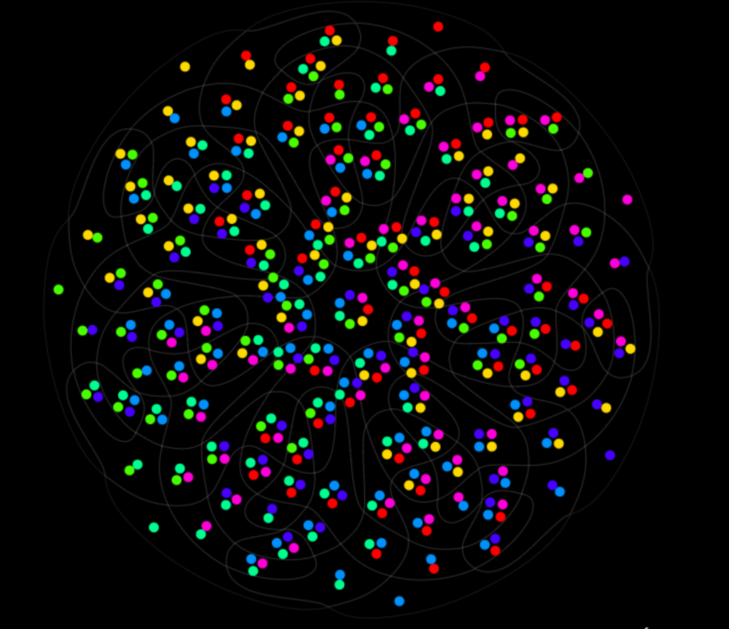
We feel fine” project was created by Jonathan Harris in 2009 for a book co-authored with Seth Kamvar. The graphs show in-depth exploration of human emotions. They’re developed from a database of more than twelve million individual sentences collected over three years from personal blogs on the Internet and show the world’s emotional landscape of ups and downs. I personally admire how he was able to create a statistical graph of the world’s emotional struggles, such as mood swings. I thought that choosing this particular theme was interesting to begin with. I believe that gathering information on emotional state and putting it into graphs are more challenging than getting statistical and measurable information, such as rainfall rate, and turning that into graphs. His artistic ability shined through his graph by using different color schemes and styles to convey all the different emotions. His graphs clearly conveyed the complexity of emotions as well.

One of the “We feel fine” graphs

Project-07 Curves

sketch

//Robert Rice
//rdrice
//Section C

var x=[];       //bucket of x-coordinates for the vertices
var y=[];       //bucket of y-coordinates for the vertices
var a = 26.5;   //The scale of the curve
var n = 200;    //The curve's "resolution". How many vertexes are used to form the curves.
var q = 3;      //the number of petals

var rStart = 0;
var angle = 0;  //variable that contains the slow, global rotation
var dr = .1;    //speed of slow rotation

function setup() {
    createCanvas(480, 480);
    background(220);
    angleMode(DEGREES);  //me dum dum no like radians
}

function draw() {
    background(0);
    translate(width/2, height/2);   //sets center of the drawng to the center of the canvas
    stroke(255);
    strokeWeight(1);
    noFill();

    q = map(mouseY, 0, height, 3, 30, true);
    a = map(mouseX, 0, width, -26.5, 26.5, true);
    rStart = map(mouseY, 0, height, 0, 360);

    for (i= 0; i < n; i++) {    //calculates the base curve x and y-values
        let t = -10 + (20/n)*i  //calculates 't' values that are used to evaluate x and y components
        x[i] = 3*a*((t**2) - 3);
        y[i] = a*t*((t**2) - 3);
    }

    for (let i = 0; i < q; i+=1) {
        petal(0, 0, rStart+angle+i*(360/q));
    }

    angle = angle + dr  //drives the rotation of the drawing
}

function petal(v, w, r) {
    push();
    translate(v, w);
    rotate(r);

    beginShape()
    for (i=0; i < n; i++) {
        vertex(x[i], y[i]);
    }
    endShape();
    pop(); //forms a petal at v(x-coord) and w(y-coord) with rotation r based on the curve defined in line 25
}

Project 07: Curves

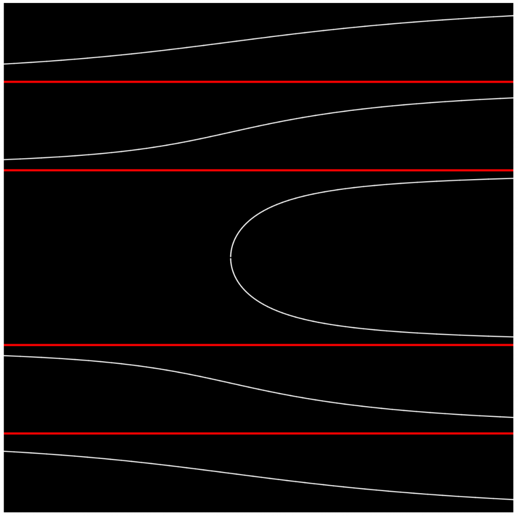
For this assignment I began with the equation for the Quadratrix of Hippias, and scaled the equation based on the Y-Coordinate of the mouse. I also identified the limits of the formula and changed their visibility based on the X-Coordinate of the mouse.

sketchDownload
var t = 0;
var points = 200;
var eX = [];
var eY = [];
var a = 0;
var b = 0;
var r = 200;

function setup() {
    createCanvas(480, 480);
    background(0);

    stroke(255);
    strokeWeight(1);
    noFill();

    a = 15;
    b = mouseY;
}

function draw() {
  background(0);

  if (mouseY < 150 || mouseY > 330) {
    a = map(mouseY,0,height,-40,40);
  } else {a = 15}

  for (let i = 0; i < height; i += 1) {
    eY[i] = i;

    eX[i] = eY[i]*((1)/(tan((PI*eY[i])/(2*a))));

    line(eX[i]+240,eY[i]+240,eX[i+1]+240,eY[i+1]+240);
    line(eX[i]+240,-eY[i]+240,eX[i+1]+240,-eY[i+1]+240);

    if (abs((eX[i])-(eX[i+1])) > 400) {
      push();
      strokeWeight(2);
      stroke(map(mouseX,0,width,0,255),0,0);
      line(eX[i]+240,eY[i]+240,eX[i+1]+240,eY[i+1]+240);
      line(eX[i]+240,-eY[i]+240,eX[i+1]+240,-eY[i+1]+240)
      pop();
    }
  }
}

Looking Outwards 07: Information Visualization

Of the examples I looked at, I really enjoyed the 7 sets Venn Diagram, made by Santiago Ortiz’s Moebio Labs. I really like that they use colors instead of numbers or letters, since it makes the intersections between the different sets much simpler to understand. The work was created by looking at a static set of the 7 way Venn Diagram, and using the shapes as a base to create an interactive version. Similar to much of the other work on the Moebio website, they use a lot of color, specifically intersections of color, in order to help with visualization and gradients between zones. I think that it is also great that they didn’t stop at the first success, and went on to add a second side of the diagram which consists of only the gradients of different colors.

Project 07-Curves

sketch
var nPoints = 100;
function setup() {
    createCanvas(400, 400);
    frameRate(60);
}


function draw() {
    background(0);
    
    // draw the frame
    fill(0); 
    noStroke();
    stroke(57,255,20);
    noFill(); 
    rect(0, 0, width-1, height-1); 
    
    // draw the curve
    push();
    translate(width / 2, height / 2);
    for( var count = 1; count <= 9; count += 1){
      if(count <=3){
        drawButterflyCurve(-200 + count*100, 110);
      }else if(count <= 6){
        drawButterflyCurve(-200 + (count-3)*100, 0);
      }else if(count <= 9){
        drawButterflyCurve(-200 + (count - 6)*100, -110);


      }
    }
    pop();
  
}
function drawButterflyCurve(dx, dy){
  var x;
  var y;
  beginShape();
  for (var i = 0; i < nPoints; i++) {
        var t = map(i, 0, nPoints, 0, TWO_PI);
        x = 20*Math.sin(t) * [(Math.E)**(Math.cos(t)) - 2*Math.cos(mouseX/100 + 4*t) + (Math.sin(t/12))**5] - dx;
        y = -20*Math.cos(t) * [(Math.E)**(Math.cos(t)) - 2*Math.cos(mouseY/100 + 4*t) + (Math.sin(t/12))**5] - dy;
    vertex(x,y);
    
  }
  endShape(CLOSE);
}

Reading the project description, I was very intimidated by this week’s project due to all the complicated formulas and many options. I think I was drawn to the butterfly curve because of the shape and the complexity of it. I wanted to make a pattern out of these curves while it would turn based off the mouse’s position. Based on the mouse position, the curves would change and the lines would make different positions.

Project 07 : Curves

petal
//Rachel Kim
//15-104(Section C)
//rachelki@andrew.cmu.edu
//Project 07


//global variables
var numPoints = 800;

function setup() {
    createCanvas(480, 480);
}

function draw() {
    
    background(200); //dusty pink bkgrd color
    

    for (var x = 40; x <= 480; x += 80) {	//number of "modules" (grid)
        for (var y = 40; y <= 480; y += 80) {
            push();
            translate(x, y);
            EpicycloidPedal();
            pop();
        }
    }

    for (var x = 80; x <= 460; x += 80) {	//number of "modules" (grid)
        for (var y = 80; y <= 460; y += 80) {
            push();
            translate(x, y);
            HypocycloidPedal();
            pop();
        }
    }
}


function HypocycloidPedal() {
    
    //radius
    var a = map(mouseX, 0, 480, 0, 120); 
    var b = map(mouseX, 0, 480, 0, 60);

    strokeWeight(mouseY/100, mouseX/350); //change in stroke thickness
    stroke(158, 188, 254); //blue color
    noFill();

    //moduleShape
    beginShape();
    for (var i=0; i<numPoints; i++) {
        var angle = map(i, 0, 180, 0, TWO_PI);
        var n = 8; //number of pedals

        //equations from mathworld
        x = a * (((n-1) * cos(angle)) + (cos((n-1) * angle)) / n);
        y = a * (((n-1) * sin(angle)) - (sin((n-1) * angle)) / n);

        vertex(x, y);    	
    }
    endShape(); 	
}


function EpicycloidPedal() {

    //radius
    var a = map(mouseX, 0, 480, 0, 160); 
    var b = map(mouseX, 0, 480, 0, 80); 


    strokeWeight(mouseX/80, mouseY/200); //change in stroke thickness
    stroke(255, 242, 147); //yellow color
    noFill();

    //module shape
    beginShape();
    for (var i=0; i<numPoints; i++) {
        var angle = map(i, 0, 100, 0, TWO_PI);

        //equations from mathworld
        x = ((1/2) * (a+(2*b))) * (cos(angle) - cos(((a+b)*angle) / b));
        y = ((1/2) * (a+(2*b))) * (sin(angle) - sin(((a+b)*angle) / b));

        vertex(x, y);
    }
    endShape();

}

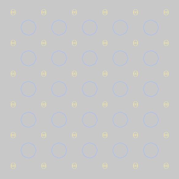
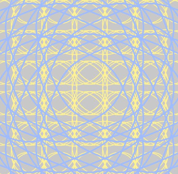
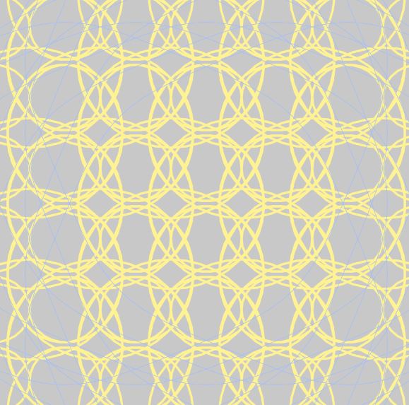
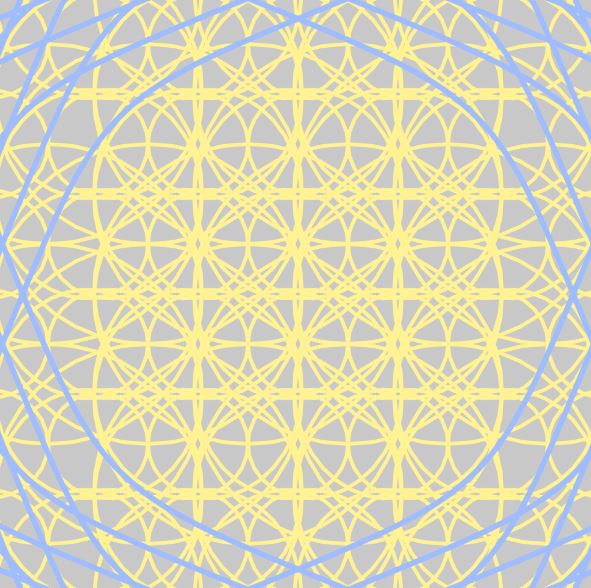
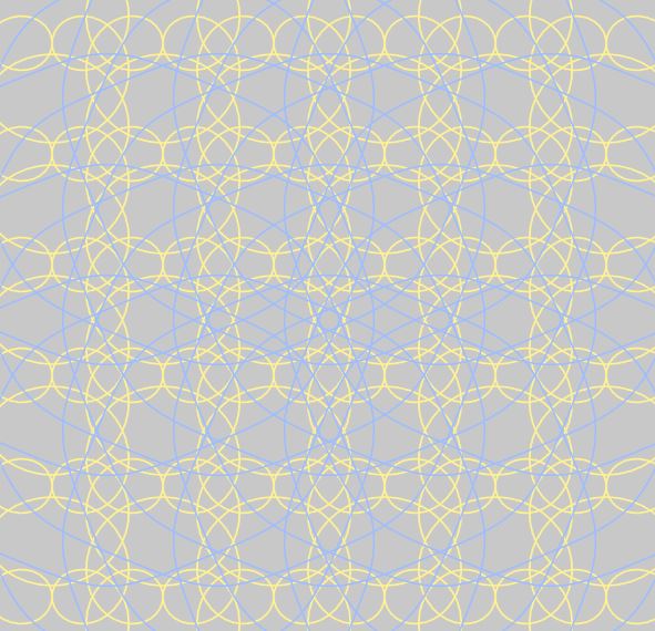
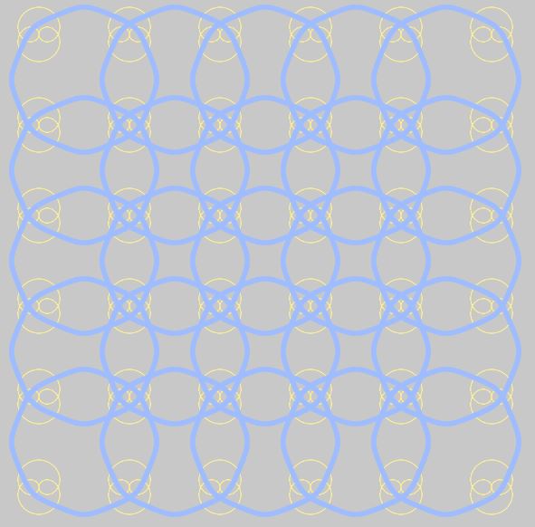
After browsing through the Mathworld curves site, I wanted to explore the possibilities of the Hypocycloid pedal curve and the Epicycloid pedal curve under the roulettes category. Using different functions, I tried showing the different shapes each curve had the ability to make, through the manipulation of its radius and x and y coordinates. Above, there are screenshots of the different visuals depending on where the mouse is placed on the screen. I did not want to manipulate any change in the colors, because I want the user to focus on the different geometries.

Looking Outwards 07 : Computational Information Visualization

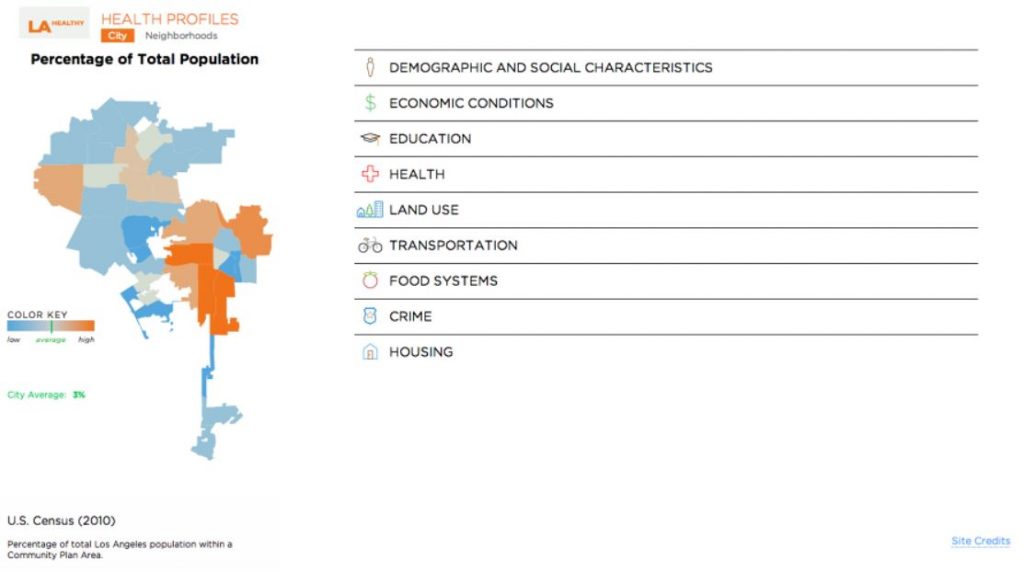
Rachel Binx is an American designer, data visualizer, and developer. She graduated from Santa Clara University and is currently the co-founder of Meshu and Gifpop. Meshu and Gifpop are companies that focus on creating visualizations from social data. One of her projects includes Healthy Los Angeles. This project’s purpose was to provide the residents of Los Angeles with a more interesting way to view information about neighborhoods. Combining creativity/art with data/numbers is a great way to grab the attention of the audience. It can also have the possibility of making information much easier to read and understand. The website itself is able to collect 100 health indicators while featuring two different views: a city-level view and a neighborhood view.

Project 7

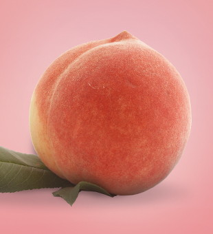
After exploring the variety of equations on the MathWorld site, I decided to use a heart curve to create peaches. My peaches are inspired by Japanese peaches, and they change color and size based on mouseX.

peaches
Japanese peach
function setup() {
    createCanvas(480, 480);
}

function draw() {
    background(150, 240, 210); //mint background
    //4 peaches
    for (var x = 140; x <= width; x += 200) {
        for (var y = 140;y <= height; y+= 200) {
        push();
        leaf(x, y);
        pop();
        push();
        translate(x, y);
        peach();
        pop();
        }
    }
}
function leaf(x, y){
    push();
    stroke(35, 153, 139);
    strokeWeight(2);
    strokeCap(SQUARE);
    fill(50, 200, 180);
    arc(x+15, y+15, 70, 40, PI/4, PI + PI/3, OPEN);
      //arc(width/220 - 25, height/2, 40, 40, PI-PI/3, , OPEN);
    pop();
  
}
function peach(){
    var colorshift = constrain(mouseX, 5, 50);
    fill(255, 180- colorshift/4, 120+colorshift/2);// peach become redder based on mouseX
    stroke(250, 250, 250); //offwhite outline
    scale(2.5);//no need to rotate peach shape
    beginShape();
    for (var i = 0; i < 2*PI; i+=0.1) {
        var mx = constrain(mouseX/300, 0.7, 1.2); //mouseX multiplier
        var x = mx*20*pow(sin(i),3);
        var y = mx*20*cos(i)-4*cos(2*i)-2*cos(3*i);
        vertex(x,y); 
    }
    endShape();
}