Project-07

sketch
//Diana McLaughlin, dmclaugh@andrew.cmu.edu, Section A
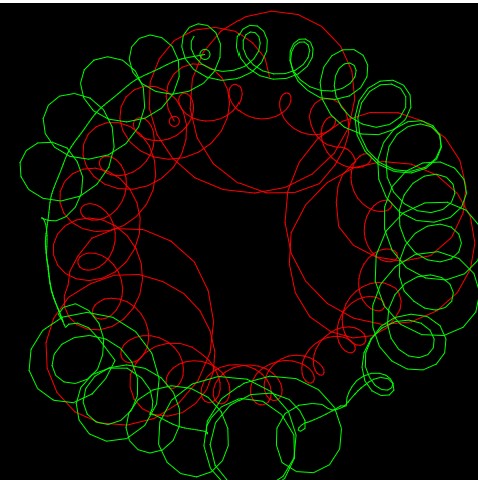
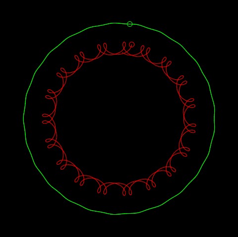
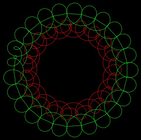
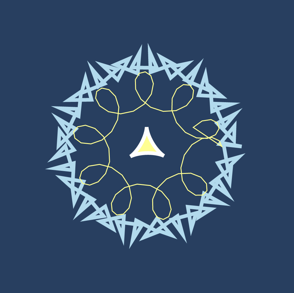
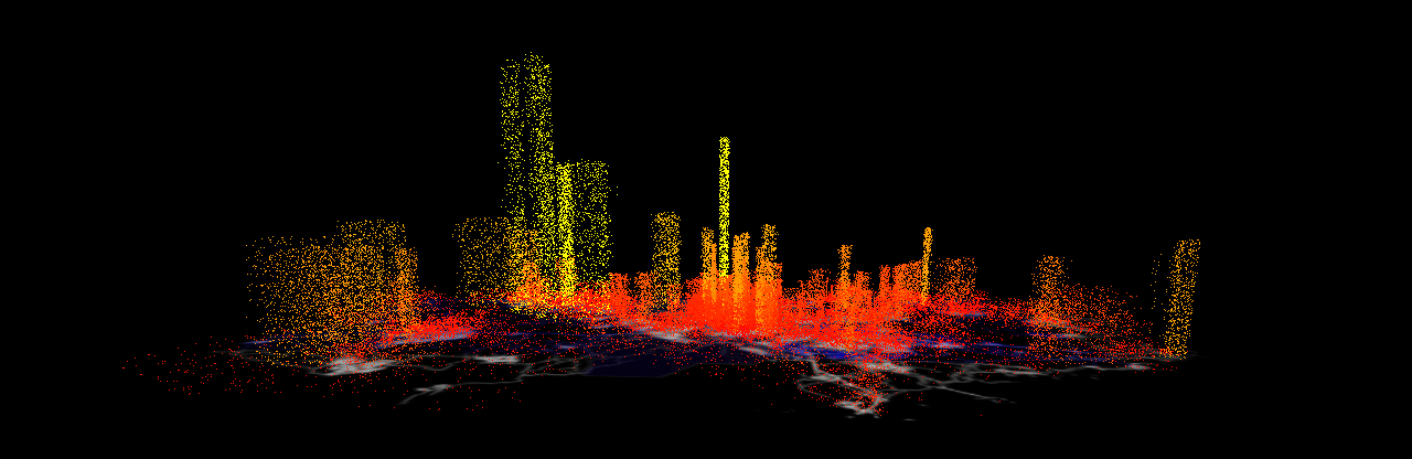
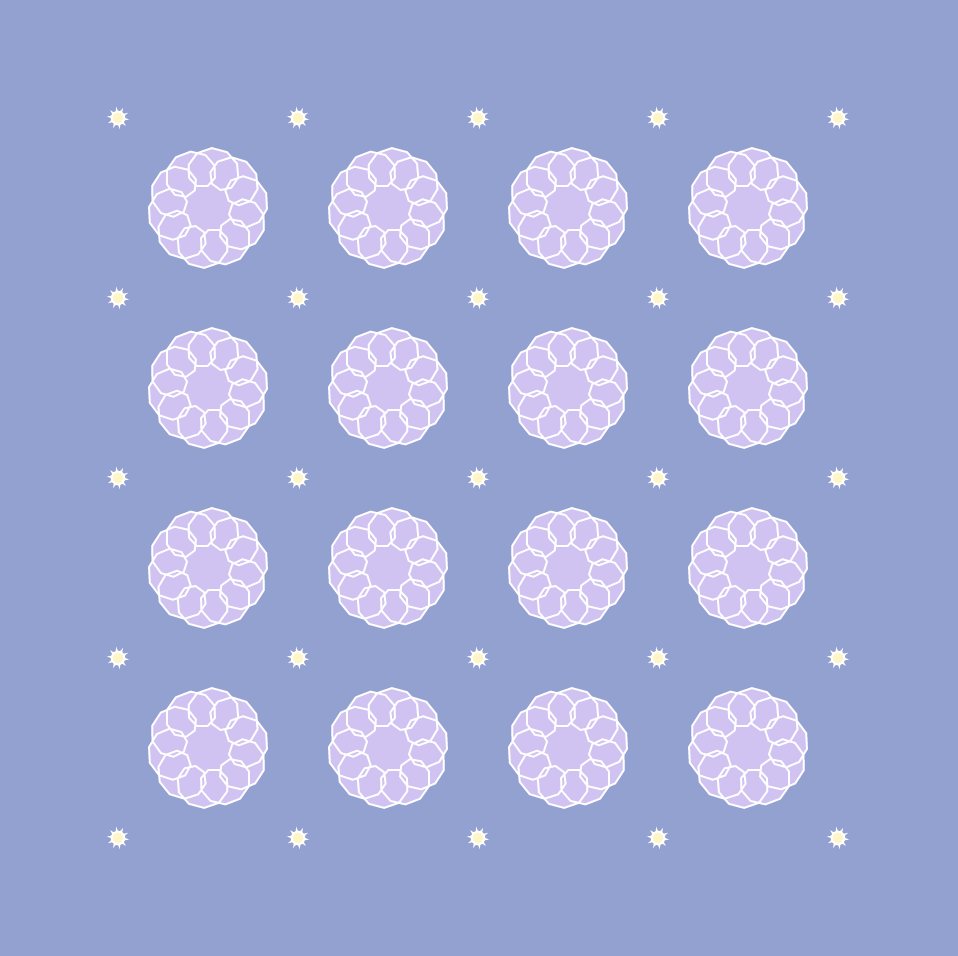
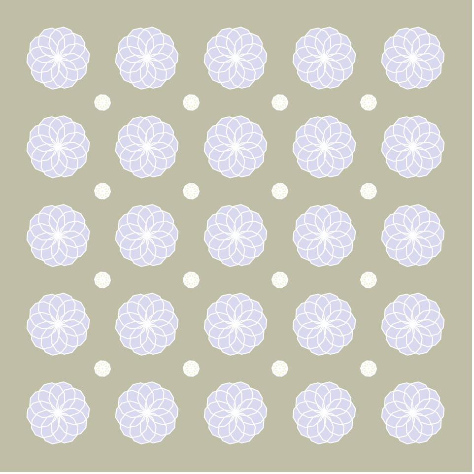
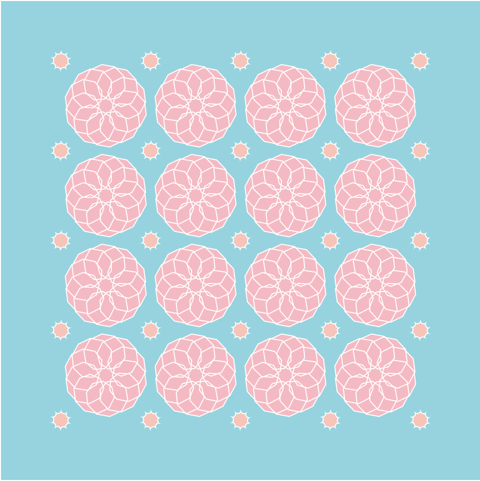
//a code that experiments with epicycloids and hypotrochoids

var nPoints = 500;
var theta = 0;

function setup() {
    createCanvas(480, 480);

}

function draw() {
	var g = map(mouseX, 0, 480, 0, 160);
	var b = map(mouseX, 0, 480, 75, 255);
    background(0, g, b); //shades of blue

    for(var y = 0; y <= 480; y += 100) { //draw the vertical yellow epicycloids
    	push();
    	translate(0, y);
    	Epicycloid2();
    	pop();
    	push();
    	translate(480, y);
    	Epicycloid2();
    	pop();
    }

    for (var x = 20; x <= 480; x += 100) {
    	    push(); //top row, yellow epicycloids
    	    translate(x, 0);
    	    Epicycloid2(); 
    	    pop();
            push(); //second row, pink hypotrochoids
            translate(x, 120);
            Hypotrochoid1();
            pop();
            push(); // middle row, purple epicycloids
    	    translate(x, 240);
    	    Epicycloid1();
    	    pop();
            push(); //fourth row, green hypotrochoids
            translate(x, 360);
            Hypotrochoid2();
            pop();
            push(); //bottom row, yellow epicycloids
            translate(x, 480);
            Epicycloid2();
            pop();

    }

    
}

function Epicycloid1() { //purple epicycloid
    var a = map(mouseX, 0, 480, 0, 70); //inner radius
    var b = map(mouseY, 0, 480, 0, 20); //outter radius

    strokeWeight(1);
    stroke(255, 128, 255); //light purple
    noFill();
    beginShape();
    for (var i = 0; i < nPoints; i++) {
        var theta = map(i, 0, 125, 0, TWO_PI);
        x = (a+b) * cos(theta) - b * cos(((a+b)/b) * theta);
        y = (a+b) * sin(theta) - b * sin(((a+b)/b) * theta);
        vertex(x, y);
    }
    endShape();
}

function Epicycloid2() { //yellow, epicycloid, used for the border
    var a = map(mouseX, 0, 480, 0, 30); //inner radius
    var b = map(mouseY, 0, 480, 0, 20); //outter radius

    strokeWeight(0.75);
    stroke(255, 255, 0); //yellow
    noFill();
    beginShape();
    for (var i=0; i<nPoints; i++) {
        var theta = map(i, 0, 45, 0, TWO_PI);
        x = (a+b) * cos(theta) - b * cos(((a+b)/b) * theta);
        y = (a+b) * sin(theta) - b * sin(((a+b)/b) * theta);
        vertex(x, y);
    }
    endShape();
}


function Hypotrochoid1() { //pink hypotrochoid
    var a = map(mouseX, 0, 480, 0, 125); //outter radius
    var b = map(mouseY, 0, 480, 0, 50); //inner radius
    var h = map(mouseX, 0, 480, 0, 60); // tracing distance from center of inner circle

    strokeWeight(1);
    stroke(255, 128, 200); //pink
    noFill();
    beginShape();
    for (var i=0; i<nPoints; i++) {
        var theta = map(i, 0, 120, 0, TWO_PI);
        x = (a-b) * cos(theta) + h * cos(((a-b)/b) * theta);
        y = (a-b) * sin(theta) - h * sin(((a-b)/b) * theta);
        vertex(x, y);
    }
    endShape();
}

function Hypotrochoid2() { //green hypotrochoid
    var a = map(mouseX, 0, 480, 0, 100); //outter radius
    var b = map(mouseY, 0, 480, 0, 40); //inner radius
    var h = map(mouseY, 0, 480, 0, 60); //tracing distance from center of inner circle

    strokeWeight(1);
    stroke(0, 255, 0);
    noFill();
    beginShape();
    for (var i=0; i<nPoints; i++) {
        var theta = map(i, 0, 120, 0, TWO_PI);
        x = (a-b) * cos(theta) + h * cos(((a-b)/b) * theta);
        y = (a-b) * sin(theta) - h * sin(((a-b)/b) * theta);
        vertex(x, y);
    }
    endShape();
}

I made this as a way to mess around with hypotrochoids and epicycloids. It took awhile to figure out the math and variables, but once I did, it was fun to play around with. The top pink row is my favorite.

Looking Outwards 07: Information Visualization

A work of computational information visualization that I find intriguing is Stamen Design’s “Metagenomics with the Banfield Lab.” This project came about when the Banfield Lab asked Stamen Design to visualize their data about gene sequences in an ecosystem. I admire the clarity of the visual result because it takes what would normally be considered complex data and arranges it in a way that is easy to access and read. I suppose that the artwork was generated by sorting the data into a matrix and visualizing the data as squares. Stamen Design’s artistic sensibilities are manifested in the final form because they created a clear and readable visualization of data while being visually interesting.

Gif of Stamen Design’s “Metagenomics with the Banfield Lab”

Project 7

After exploring the variety of equations on the MathWorld site, I decided to use a heart curve to create peaches. My peaches are inspired by Japanese peaches, and they change color and size based on mouseX.

peaches
Japanese peach
function setup() {
    createCanvas(480, 480);
}

function draw() {
    background(150, 240, 210); //mint background
    //4 peaches
    for (var x = 140; x <= width; x += 200) {
        for (var y = 140;y <= height; y+= 200) {
        push();
        leaf(x, y);
        pop();
        push();
        translate(x, y);
        peach();
        pop();
        }
    }
}
function leaf(x, y){
    push();
    stroke(35, 153, 139);
    strokeWeight(2);
    strokeCap(SQUARE);
    fill(50, 200, 180);
    arc(x+15, y+15, 70, 40, PI/4, PI + PI/3, OPEN);
      //arc(width/220 - 25, height/2, 40, 40, PI-PI/3, , OPEN);
    pop();
  
}
function peach(){
    var colorshift = constrain(mouseX, 5, 50);
    fill(255, 180- colorshift/4, 120+colorshift/2);// peach become redder based on mouseX
    stroke(250, 250, 250); //offwhite outline
    scale(2.5);//no need to rotate peach shape
    beginShape();
    for (var i = 0; i < 2*PI; i+=0.1) {
        var mx = constrain(mouseX/300, 0.7, 1.2); //mouseX multiplier
        var x = mx*20*pow(sin(i),3);
        var y = mx*20*cos(i)-4*cos(2*i)-2*cos(3*i);
        vertex(x,y); 
    }
    endShape();
}

Project 07 – Composition with Curves

I wasn’t really inspired by anything this time but I had an idea in mind of a rotating curve that had a trailing effect. I ended up with a variable epicycloid curve, formed by a point traced by a circle’s radius as it rotates around a larger circle. Clicking on the screen adds “petals” to the shape of the curve. At first, I wanted to experiment with a reuleaux triangle and make an animation similar to a rotary engine, but couldn’t figure out the math behind making the triangle follow an eccentric path.

sketch

/*
 * Eric Zhao
 * ezhao2@andrew.cmu.edu
 *
 * Interactive composition with epicycloid curves
 * that changes color with a gradient effect. Click
 * to increase the number of "petals" on the curves.
 *
 */
var numPoints = 75;
var thetaCanvas = 0;
var rotateSpeed = 2;
var multiplier = 2;
var totalScale;
var epicycloid = [];
var baseFill;

function setup() {
    createCanvas(480, 480);
    background(220);
    strokeWeight(2);
    fill(0);
    angleMode(DEGREES);
    colorMode(HSB);
}

function draw() {
        for (let i = 0; i < 10; i++){
        //creates series of nested epicycloid curve objects
        epicycloid[i] = new Object();
        epicycloid[i].shapeScale = 1 - i/10;
        epicycloid[i].a = epicycloid[i].shapeScale * 100;
        epicycloid[i].b = epicycloid[i].a / multiplier;
        epicycloid[i].theta = 0;
    }

    totalScale = map(sin(thetaCanvas), -1, 1, 0.33, 1);
    //makes composition zoom in and out smoothly
    background(0);

    push();
    translate(width/2, height/2);
    rotate(thetaCanvas);
    scale(totalScale);
    for (let i = 0; i < epicycloid.length; i++){
        //slightly offsets hue and rotation of each successive curve
        push();
        rotate(i*10);
        baseFill = ((thetaCanvas + i*10)*2) % 360;
        stroke(baseFill, 100, 100);
        epicycloidCurve(epicycloid[i]);
        pop();
    }
    pop();
    thetaCanvas += rotateSpeed;
}
function epicycloidCurve(e){
    //Epicycloid curve equation
    beginShape();
    for(let i = 0; i <= numPoints; i++){
        e.theta = map(i, 0, numPoints, 0, 360);
        e.x = ((e.a + e.b) * cos(e.theta) - e.b * cos(((e.a + e.b)/e.b) *
        e.theta));
        e.y = ((e.a + e.b) * sin(e.theta) - e.b * sin(((e.a + e.b)/e.b) *
        e.theta));
        curveVertex(e.x, e.y);
    }
    endShape(CLOSE);
}

function mousePressed(){
    //changes number of "petals" in the epicycloid
    multiplier++;
    if(multiplier > 5){
        multiplier = 2;
    }
}


Project 7 Curves Composition

There are two hypotrochoids that are being drawn simultaneously in this program, as Mouse Y changes you can alter the pedals of the hypotrochoids., the lines redraw themselves every 3 loops around the circle so as you move Mouse Y around you begin to get an overlay of various patterns.

sketch
//tjchen 
// section a 
// 07 project composisiton with curves
var t = 0
var numPoints = 100;// global set up of num of points on circle
var lineX = [];
var lineY = [];
var lineX2 = [];
var lineY2= [];
function setup() {
    createCanvas(480, 480);
    background(0);
    strokeWeight(1);
    stroke(255);
    noFill();
}


function draw() {
    background(0);
    translate(width/2,height/2)
    stroke(255,0,0);
    draw_hypotrochoid_1(t);
    stroke(0,255,0);
    draw_hypotrochoid_2(t);
    t+=1; 
}


function draw_hypotrochoid_1(t){
    var a = 150; // radius of large circle 
    var b = 8; // radius of spinning circle 
    var h = mouseY/10; // location of fixed point 
    var xH= (a-b) * cos (radians(t)) + h * cos(((a-b)/b)*(radians(t)));
    var yH = (a-b) * sin (radians(t)) - h * sin(((a-b)/b)*(radians(t))); 
    circle(xH,yH,10);;
    lineX.push(xH);
    lineY.push(yH);
    if (radians(t)>4*PI){ // 4 trips around the circle before redrawing circle 
        lineX.shift();
        lineY.shift();
    }
    strokeWeight(1);
    for (i=0; i < lineX.length-1; i++){
        line(lineX[i], lineY[i], lineX[i+1], lineY[i+1]);
    }


} 

function draw_hypotrochoid_2(t){
    var a2 = 200; // radius of large circle 
    var b2 = 8; // radius of spinning circle 
    var h2 = mouseX/10; // location of fixed point 
    var xH2= (a2-b2) * cos (radians(t)) + h2 * cos(((a2-b2)/b2)*(radians(t)));
    var yH2 = (a2-b2) * sin (radians(t)) - h2 * sin(((a2-b2)/b2)*(radians(t))); 
    circle(xH2,yH2,10);;
    lineX2.push(xH2);
    lineY2.push(yH2);
    if (radians(t)>4*PI){ // 4 trips around the circle before redrawing circle 
        lineX2.shift();
        lineY2.shift();
    }
    strokeWeight(1);
    for (i=0; i < lineX2.length-1; i++){
        line(lineX2[i], lineY2[i], lineX2[i+1], lineY2[i+1]);
    }


} 
the Circle transitioning
curves in one composition

curves in another composition

Project 07 – Composition with Curves

sketch
// Stefanie Suk
// 15-104 Section D

var nPoints = 100; //number of points for curves
var angle = 10; //angle of rotation

function setup() {
    createCanvas(480,480);
    frameRate(15); //set frame rate to 15
}

function draw() {
    background(33, 63, 99); //background of canvas to dark blue

    //placing Hypocycloid in center
    push();
    translate(width/2, height/2);
    Hypocycloid();
    pop();

    //placing Deltoid in center and rotate by angle
    push();
    translate(width/2, height/2);
    rotate(radians(angle));
    angle += mouseX;
    Deltoid();
    pop();

    //placing Epitrochoid in center
    push();
    translate(width/2, height/2);
    Epitrochoid();
    pop();
}

function Hypocycloid(){
    // variables for Hypocycloid
    var a1 = map(mouseY, 0, 300, 150, 180); //size changes with respect to mouseY
    var b1 = 15;
    var c1 = mouseX / 25;

    //color, stroke of Hypocycloid
    stroke(167, 219, 239);
    strokeWeight(6);
    noFill();

    //create curve, map to full circle radians
    //use math function to find x and y values
    beginShape();
    for (var i = 0; i < nPoints; i++) {
        var angle1 = map(i, 0, nPoints, 0, TWO_PI);     
        x1 = (a1 - b1) * cos(angle1) + c1 * cos((a1 - b1) * angle1);
        y1 = (a1 - b1) * sin (angle1) - c1 * sin((a1 - b1) * angle1);
        vertex(x1, y1);
    }
    endShape(CLOSE); 
}

function Deltoid(){
    colorR = map(mouseX, 0, 50, 100, 255);
    colorG = map(mouseX, 0, 50, 100, 255); //set color in specific range
    colorB = map(mouseY, 0, 50, 100, 255); //changes color with respect to mouseX,Y
    
    // variable for Deltoid, change size
    a2 = map(mouseY, 0, height, 10, 40); //size changes with respect to mouseY
    
    //color, stroke, fill of Deltoid
    stroke(255);
    strokeWeight(6);
    fill(colorR, colorG, colorB);

    //create curve, map to full circle radians
    //use math function to find x and y values
    beginShape();
    for (var i = 0; i < nPoints; i++) {
        var angle2 = map(i, 0, nPoints, 0, TWO_PI);
        x2 = ((2 *(cos(angle2))) + (cos(2*angle2)))* a2 ;
        y2 = ((2 *(sin(angle2))) - (sin(2*angle2)))* a2 ;
        vertex(x2, y2);
    }
    endShape(CLOSE);
}

function Epitrochoid() {

    colorR = map(mouseX, 0, 50, 100, 255);
    colorG = map(mouseX, 0, 50, 100, 255); //set color in specific range
    colorB = map(mouseY, 0, 50, 100, 255); //changes color with respect to mouseX,Y

    // variables for epitrochoid
    var a3 = map(mouseY, 0, 400, 40, 110); //size changes with respect to mouseY
    var b3 = 50;
    var c3 = (mouseX / 15);

    //color, stroke of epitrochoid
    stroke(colorR, colorG, colorB);
    strokeWeight(1.5);
    noFill();

    //create curve, map to full circle radians
    //use math function to find x and y values
    beginShape();
    for (var i = 0; i < nPoints; i++) {
        var angle3 = map(i, 0, nPoints, 0, TWO_PI);
        x3 = (a3 + b3) * cos(angle3) + c3 * cos((a3 + b3) * angle3);
        y3 = (a3 + b3) * sin(angle3) + c3 * sin((a3 + b3) * angle3);
        vertex(x3, y3);
    }
    endShape(CLOSE);
}

I utilized hypocycloid, deltoid, and epitrochoid using the reference from Mathworld to create this project. I chose these curves because I loved how they were structured. I thought that when these three curves are put together would create one unique interactive shape for my project. The exploration of this project was interesting, and I also played around with random colors and sizes with mouseX and mouseY. The unique part about these curves in my project is that the curves in my work create different smoothness depending on the position of the mouse (round, shape, spiky, squiggly). The different shapes created in the project look like forms of snowflakes, which is why I made the main color blue.

LO-07: Information Visualization

The project I chose this week was Aaron Koblin’s Amsterdam SMS. This project is an interactive visualization tool developed for the MIT Senseable City Lab which helps visualize SMS messages data. I admired this project because I was drawn to the boldness of the colors and like any artwork done using data, I just thought it was very interesting and cool. To generate this work, Koblin used Processing and OpenGL. The data he used was provided by KPN Mobile. Like his other works, Koblin uses bright colors or “light” (he doesn’t actually use light in this project but the bright colors do give off a similar effect!) to stimulate our sight and draw attention to the artwork.

Video of Amsterdam SMS Messages on New Years Eve (2007)

Project-07: Curves

For this week’s project, I decided to use 2 different curves that reminded me of flowers, a 10 cusp Epicycloid and a 10 cusp Hypotrochoid. I decided to make them rotate and change in size based on the mouse movements but in opposite directions to give off a pulsating effect. I also utilized mousePressed so that the curves can alternate. The mouse positions also control the colors of the curves and the background so that the final output is unique in all positions. The colors of the flowers and background are quite muted to give off a slight vintage wallpaper vibe with a modern twist.

(below are screenshots of the code at different mouse positions)

sketch

function setup() {
    createCanvas(480, 480);
}

var nPoints = 100;

// background color codes
var r = 205;
var g = 152;
var b = 152;

// to switch curves based on mouse click
var whichCurve = 0;

// curve color codes
var curver = 202;
var curveg = 255;
var curveb = 255;

function draw() {

	// to add/subtract color codes based on mouse position
	var colordiffX = map(mouseX, 0, 480, 0, 53);
	var colordiffY = map(mouseY, 0, 480, 0, 53);

	background(r - colordiffX, g + colordiffY, b + colordiffX);

	stroke(255); // white outline

	// 5 x 5 curves (outer)
	for(var x = 60; x < width; x += 90){
		for(var y = 60; y < height; y += 90){
			push();
			translate(x, y);
			fill(curver + colordiffX, curveg - colordiffY, curveb - colordiffX);
			if(whichCurve == 0) {
				drawHypotrochoid();
			}
			else {
				drawEpicycloid();
			}
			pop();
		}
	}
	// 4 x 4 curves (inner)
	for(var x = 105; x < width - 90; x += 90) {
		for(var y = 105; y < height - 90; y += 90) {
			push();
			translate(x, y);
			fill(curver + colordiffY, curveg - colordiffX, curveb - colordiffY);
			if(whichCurve == 1) {
				drawHypotrochoid();
			}
			else {
				drawEpicycloid();
			}			
			pop();
		}
	}
}

// draw rotating 10 cusp epicycloid
function drawEpicycloid() {
	var x;
	var y;
	var a = mouseX / 30;
	var b = a / 10;
    var h = constrain(mouseY / 8, a / 10, 8*b);
    var ph = mouseX / 50;

    beginShape();
    for (var i = 0; i < nPoints; i++) {
        var t = map(i, 0, nPoints, 0, TWO_PI);
        x = (a + b) * cos(t) - h * cos(ph + t * (a + b) / b);
        y = (a + b) * sin(t) - h * sin(ph + t * (a + b) / b);
        vertex(x, y);
    }
    endShape(CLOSE);
}

// draw rotating 10 cusp hypotrochoid
function drawHypotrochoid() {
	var x;
	var y;
	var a = (width - mouseX)/20; // opposite movement from epicycloid
	var b = a / 10;
    var h = constrain((height - mouseY)/8, a/10, 10*b);
    var ph = (width - mouseX) / 50;

    beginShape();
    for (var i = 0; i < nPoints; i++) {
        var t = map(i, 0, nPoints, 0, TWO_PI);
        x = (a - b) * cos(t) + h * cos(ph + t * (a - b) / b);
        y = (a - b) * sin(t) - h * sin(ph + t * (a - b) / b);
        vertex(x, y);
    }
    endShape(CLOSE);
}

// mouse pressed alternates order of curves
function mousePressed() {
	if(whichCurve == 0){
		whichCurve = 1;
	}
	else {
		whichCurve = 0;
	}
}

Looking Outwards-07: Computational Visualization

One piece of work that I admire is Jer Thorp’s “138 Years of Popular Science.” The data compiled is from Pop Science magazine’s past publications. The chart illustrates how different scientific terms have come into and out of popular usage over the years in scientific reports. As somewhat of an homage to the content, the data is visualized in a molecular chain format, with different atoms delineating distinct year clusters, further demarcated with different colors. Thorp developed a “simple, space-filling algorithm” that places the different molecules around the chain, and stacking them deliberately to create a neat flow. Further deepening the study is layered histograms in the background, showing the usage from different issues of specific terms. I like this work because it shows the artist’s personal design style with whimsical coloring and visualization, while also respecting the client for whom they are producing for with logic and thorough analysis. Every detail was clearly thought out. Furthermore, not only is it aesthetic but intellectually intriguing as it shows a progression and shift of technology and academic focus.

In a somewhat unrelated note, in the reddit app there is a subreddit that is interesting called r/dataisbeautiful which features data visualizations by anyone (ie regular people!) who chooses to submit a post. The content ranges from “Daily Polar Sea Ice Area with Monthly Ice Extent” to “The distribution of Minecraft Biomes in the overworld.”

Project 06-Abstract-Clock

sketchDownload
var x = 0;
var y = 0;
var sDiam;

function setup() {
    createCanvas(600, 600);
}

function draw() {
    var s = second();
    var m = minute();
    var h = hour();
    background(0, 0, h*10); //gets lighter by the hour
    translate(width/2, height/2);
    minuteRing(s, m);
    secondRing(s, m, sDiam);
}

function minuteRing(s, m) { //big circle that appears within a minute
    noStroke();
    fill(148, 96, 139, s*4.25); //opacity increases with second
    circle(x, y, 10*m); //diameter increases with minute
}
 
function secondRing(s, m, sDiam) {  //the ticking clock that moves every second
    fill(148, 96, 139);
    rotate(radians(s*6)); //rotate every second by 6 degrees
    var sDiam = (PI*10*m)/60; //diameter is circumference divided by 60 secs
    circle(x+(10*m/2), y, sDiam);
    triangle(x, y, x+(10*m/2), y-(sDiam/2), x+(10*m/2), y+(sDiam/2));
}

For this project I struggled a bit because I didn’t have enough time to create what I had visualized. I was inspired by the flower that blooms at night and wanted to create an image where the pedals grow bigger and bigger as time goes on.

I was only able to get the one pedal moving instead of having the whole flower in the background but basically the circle reveals itself to full opacity every minute as the pedal rotates, then the ring diameter increases with the minute. The background blue becomes lighter by the hour to signify sky.