Timothy Liu — Project 07 — Curves

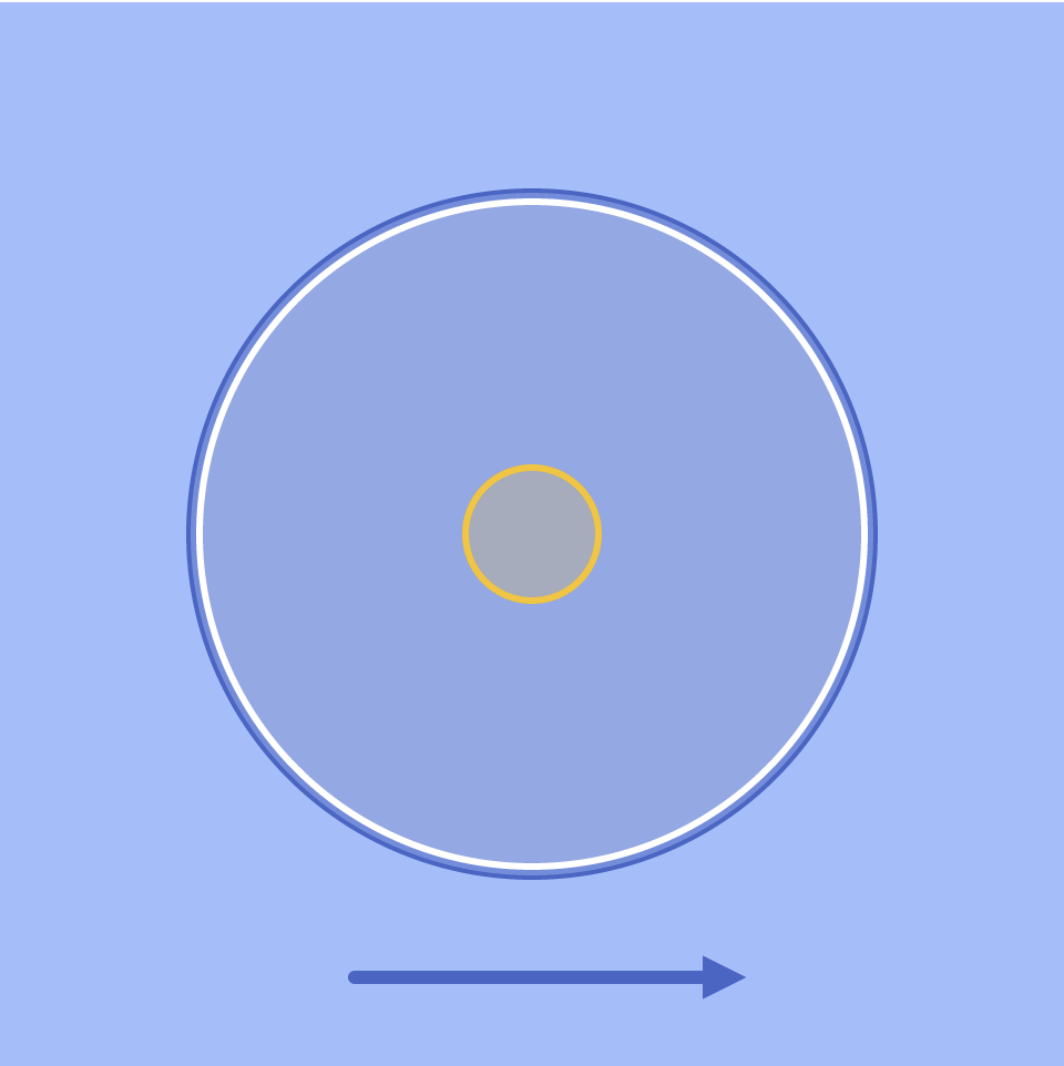
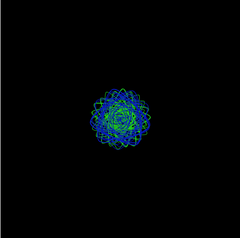
Slowly move the mouse across the canvas (from L to R) to watch the circle transform into a flower!

tcliu-openproject-07

// Timothy Liu
// 15-104, Section C
// tcliu@andrew.cmu.edu
// OpenProject-07

var nPoints = 1000; // number of points in each function. The more points, the smoother the function is.

// variables for white quadrifolium
var k;
var n;
var d;

// variables for blue quadrifolium
var k2;
var n2;
var d2;

// variables for flower center
var k3;
var n3;
var d3;

function setup() {
    createCanvas(480, 480);
    frameRate(30);
}

function draw() {
    background(160, 190, 255); // light blue background

    k = n / d; // k constant determines the number of petals on the white quadrifolium
    k2 = n2 / d2; // k constant determines the number of petals on the blue quadrifolium
    k3 = n3 / d3; // k constant determines the number of petals on the flower center

    arrow(); // drawing in the arrow function
    quadrifolium2(); // drawing in the blue flower underneath first
    quadrifolium(); // drawing in the white flower on top
    flowerCenter(); // drawing in the yellow center on top of the other two flowers
}

// the white flower/quadrifolium
function quadrifolium() {
    
    // these variables/constraints hold mouseX to the width of the canvas
    // mouseX1 slows down the speed of mouseX
    var mouseX1 = mouseX / 5;
    var mouseMove = constrain(mouseX1, 0, width / 5);

    // these variables/constants help determine the location of the flower via the equation and vertex
    var r;
    var x;
    var y;

    // n and d help determine the k constant, or the number of petals on the flower
    n = map(mouseMove, 0, width, 0, 36);
    d = 4;

    // a determines the size of the white petals
    var a = 150;

    // white flower colors
    stroke(255, 255, 255);
    strokeWeight(3);
    fill(255, 255, 255, 60);

    // drawing the white quadrifolium!
    beginShape();
    for (var i = 0; i < nPoints; i++) {

        var t = map(i, 0, nPoints, 0, TWO_PI * d); // determines theta (the angle)
       
        r = a * cos(k * t); // the equation that draws the quadrifolium

        x = r * cos(t) + width / 2; // these help compute the vertex (x, y) using the circular identity
        y = r * sin(t) + width / 2;
        vertex(x, y);
    }
    endShape();
    
}

// the blue flower/quadrifolium
function quadrifolium2() {

    // these variables/constraints hold mouseX to the width of the canvas
    // mouseX2 slows down the speed of mouseX
    var mouseX2 = mouseX / 5;
    var mouseMove2 = constrain(mouseX2, 0, width / 5);

    // these variables/constants help determine the location of the flower via the equation and vertex
    var r2;
    var x2;
    var y2;

    // n2 and d2 help determine the k2 constant, or the number of petals on the flower
    n2 = map(mouseMove2, 0, width, 0, 72);
    d2 = 6;

    // a2 determines the size of the blue petals (slightly longer than the white)
    var a2 = 155;

    // blue flower colors
    stroke(71, 99, 201);
    strokeWeight(2);
    fill(71, 99, 201, 140);

    // drawing the blue quadrifolium!
    beginShape();
    for (var u = 0; u < nPoints; u++) {
        var h = map(u, 0, nPoints, 0, TWO_PI * d2); // determine theta (the angle)

        r2 = a2 * cos(k2 * h); // the equation that draws the quadrifolium

        x2 = r2 * cos(h) + width / 2; // these help compute the vertex (x2, y2) using the circular identity
        y2 = r2 * sin(h) + width / 2;
        vertex(x2, y2);
    }
    endShape();
    
}

// the yellow center of the flower (also a smaller quadrifolium)
function flowerCenter() {

    // these variables/constraints hold mouseX to the width of the canvas
    // mouseX3 slows down the speed of mouseX
    var mouseX3 = mouseX / 5;
    var mouseMove3 = constrain(mouseX3, 0, width / 5);

    // these variables/constants help determine the location of the flower via the equation and vertex
    var r3;
    var x3;
    var y3;

    // n3 and d3 help determine the k3 constant, or the number of petals on the yellow center
    n3 = map(mouseMove3, 0, width, 0, 20);
    d3 = 5;

    // a3 determines the size of the yellow center quadrifolium
    var a3 = 30;

    // yellow center color
    stroke(247, 196, 12);
    strokeWeight(3);
    fill(247, 196, 12, 50);

    // drawing the yellow center quadrifolium!
    beginShape();
    for (var c = 0; c < nPoints; c++) {
        var e = map(c, 0, nPoints, 0, TWO_PI * d3); // determine theta (the angle)

        r3 = a3 * cos(k3 * e); // the equation that draws the quadrifolium

        x3 = r3 * cos(e) + width / 2; // these help compute the vertex (x3, y3) using the circular identity
        y3 = r3 * sin(e) + width / 2;
        vertex(x3, y3);
    }
    endShape();
    
}

// the blue arrow on the bottom that indicates which way to move the mouse... toward the right!
function arrow() {

    // variables for the line part of the arrow
    var lineH = height - 40;
    var lineS = width / 3;
    var lineE = 2 * width / 3;

    // variables for the arrowhead part of the arrow
    var arrowH1 = lineH - 5;
    var arrowHT = lineE + 10;
    var arrowH2 = lineH + 5;

    // the arrow!
    stroke(71, 99, 201);
    fill(71, 99, 201);
    strokeWeight(6);
    line(lineS, lineH, lineE, lineH);
    triangle(lineE, arrowH1, arrowHT, lineH, lineE, arrowH2);
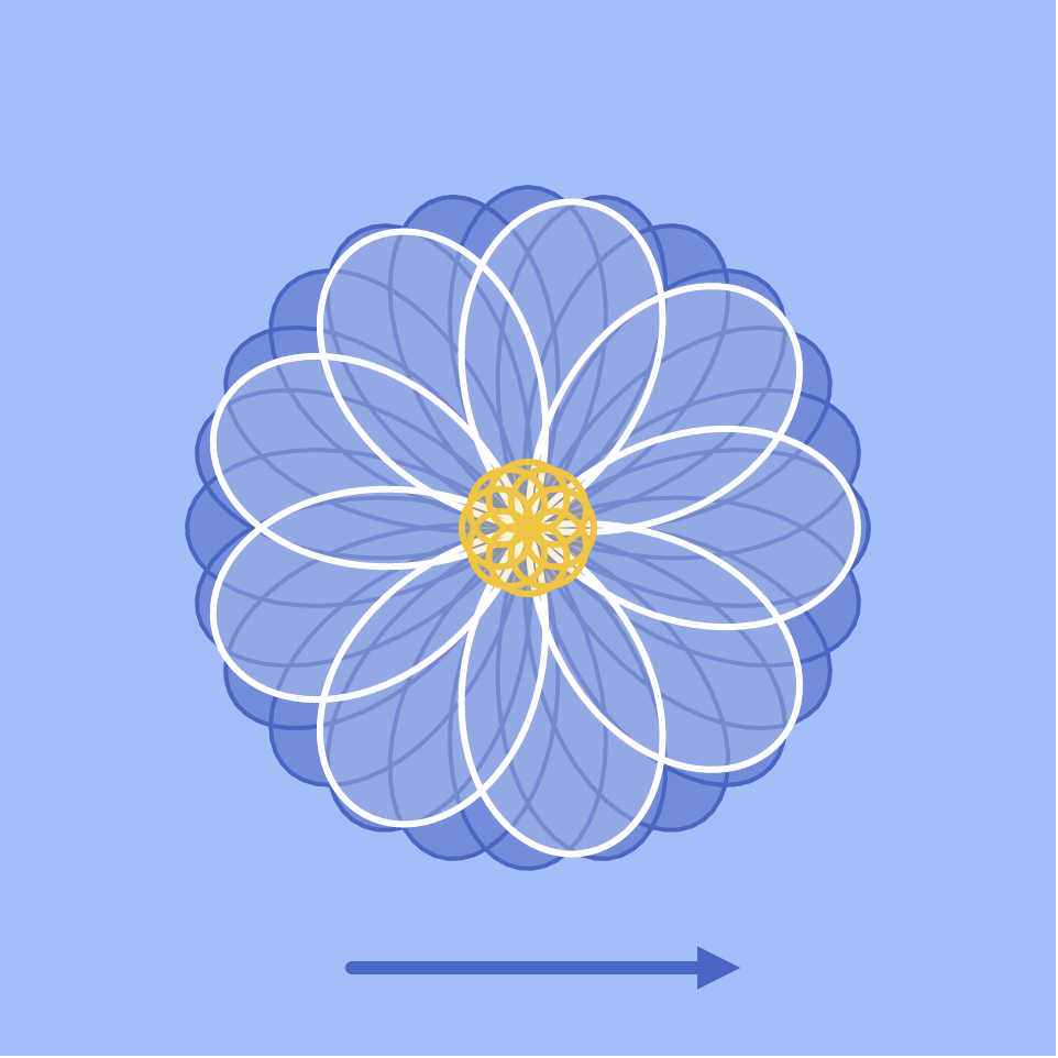
}

I struggled initially with this project because it had been so long since I mapped parametric curves in any class, let alone in a programming class. However, as I pored through Wolfram Alpha’s libraries, the Quadrifolium, or Rose Curve, immediately jumped out at me for its simplicity and elegance. I really loved how much it looked like a flower, and I thought it was really neat how the number of petals could be manipulated based on a simple constant k before the θ in the equation:

r = a * cos(kθ)

I knew that I wanted to make my quadrifolium feel like an actual flower, so I modeled my design after the blue Chrysanthemum flower.

Blue chrysanthemums, the inspiration for my flower design.

After I had drawn out the basic flower using multiple layers of quadrifolia, I decided to make my piece interactive by having the mouseX control the amount of petals on the flower. By doing so, I was able to make my design/curve “transform” from a basic circle into a beautiful flower!

The starting point of my flower…
…to the ending point, with petals!

Sarah Kang-Looking Outwards-07

“Madonna’s ‘Like a Virgin’“, by Martin Wattenberg

In this project, “The Shape of Song”, artist Martin Wattenberg demonstrates his explorations of trying to “see” musical form. I was intrigued by this project because adding a dimension of visual sense allows one to experience and interpret music in a brand new way. To achieve this experiment, Wattenberg created a visualization program that highlights the repeated verses in music using translucent arcs, called an “arc diagram”. This software, written entirely in Java. analyzes “MIDI” files of the musical piece which are commonly found on the web. Using this information, an arc connects a pair of identical sections of a musical piece. The arcs seem to be proportionally sized in terms of the spacing of the repeated sections. This allows the piece to be viewed in terms of its structure, rather than sound. The visualizations created by Wattenberg allow the viewer to analyze the entire musical piece as one visual composition in a matter of seconds, as opposed to the minutes it would take to listen to the entire song.

“Moonlight Sonata, by Beethoven” by Martin Wattenberg

http://bewitched.com/song.html

lee chu – looking outwards 07

gun death visualization by Periscope for 2013

Kim Ree, co-founder of a data visualization firm Periscopic, is probably best known for her work in visualizing gun deaths in 2010 and 2013. The diagram above illustrates the overwhelming amount of deaths from U.S. owned guns. The orange strokes depict the actual lifespans of gun victims, and the gray projects an estimated lifespan according to the U.S. distribution of deaths and likely causes of death. By also counting the amount of hours that these victims were robbed of, the data is much more impactful than if it were simply a death count. Play with the visualizer here.

Not speaking in relation to this particular piece, but I think the most interesting aspect about data visualization is that it can be depicted in a way to sway or even change one’s impressions of anything.

Jasmine Lee – Looking Outwards – 07

Created by Nathan Yau in 2017, Occupation Matchmaker is an interactive data visualization that looks at who people in certain occupations end up marrying. The project builds off an earlier project released by Adam Pearce and Dorothy Gambrell for Bloomberg.

Software developers often end up marrying within the same industry, notably to other software developers.
Original visualization by Pearce and Gambrell.

Yau’s artistic sensibility is clearly visible in the way he chose to visualized the grouping of different types of occupations and how they overlap. The visualization of this project, compared to its initial development by Pearce and Gambrell, showcase a more holistic image across the board. The viewer is made clearly aware of the connections that exist between different occupations within the same industry whereas the earlier chart shows more linear connections. In creating this visualization, Yau made sure to take into account how some occupations are much more common than others, and used a relative scale to change the sizes of the circles. Yau created this visualization using R (to analyze) and d3.js.

Musicians overwhelmingly marry other musicians, but also marry others from wildly different occupations.

lee chu – project 07 – curves

lrchu

// lee chu
// section c
// lrchu@andrew.cmu.edu
// project - 07

// variables for equation
var angle;
var t;
var x;
var y;
var xx;
var yy;

// characteristics of shapes
var sizes = [];
var size;
var ct;
var step;

// color
var r;
var g;
var b;

function setup() {
    createCanvas(480, 300);
    noFill();
    strokeWeight(0);
    angle = 0;
    t = 20;

    // create sizing for layers
    for (h = 0; h < 60; h ++) {
        sizes.push(h * 3);
    }
    size = 20;
    ct = 200;

    // color control
    r = 36;
    g = 33;
    b = 40;
    step = 5;
}

function draw() {
    background(r, g, b);

    // change turn direction and rate
    if (mouseX < width / 2 & mouseX > 0 && mouseY < height && mouseY > 0) {
        angle -= (width / 2 - constrain(mouseX, 0, width / 2)) / width / 2 / 6;
    }
    if (mouseX > width / 2 & mouseX < width && mouseY < height && mouseY > 0) {
        angle += (constrain(mouseX, width/2, width) - width / 2) / width / 2 / 6;
    }

    // generate shapes
    for (j = 0; j < sizes.length; j ++) {
        cata(sizes[sizes.length - j]);
        r = (r + step * (j + 1)) % 255;
        g = (g + step * (j + 1)) % 255;
        b = (b + step * (j + 1)) % 255;
    }
    deltoid(sizes[1]);
}

function cata(size) {
    fill(r, g, b);
    push();
    translate(width / 2, height / 2);
    beginShape();
    for (i = 0; i < ct; i ++) {
        t = map(i, 0, ct, 0, 2 * PI);
        xx = 3 * cos(t) + cos(3 * t + 2 * angle) - cos(2 * angle);
        yy = - 3 * sin(t) + sin(3 * t + 2 * angle) - sin(2 * angle);
        vertex(xx * size, yy * size);
    }
    endShape();
    pop();
}

function deltoid(sizeD) {
    fill('black');
    push();
    translate(width / 2, height / 2);
    beginShape();
    for (i = 0; i < ct; i ++) {
        t = map(i, 0, ct, 0, 2 * PI);
        x = 2 * cos(t) + cos(2 * t);
        y = -2 * sin(t) + sin(2 * t);
        vertex(x * sizeD, y * sizeD);
    }
    endShape();
    pop();
}

I was intrigued by the deltoid catacaustic, which consists of the deltoid, a triangle bowing in, and the catacaustic which circumscribes the deltoid as it rotates around its axis. The center of all the layers of the catacaustic is the black deltoid in the middle of the canvas.

Ammar Hassonjee – Project 07 – Curves

Interactive Curve Drawing

/* Ammar Hassonjee
    ahassonj@andrew.cmu.edu
    Section C
    Project 07
  */

  var nPoints = 100;
  var angle = 0;
  var angle2 = 0;
  var angle3 = 0;
  function setup() {
      createCanvas(480, 480);
  }


  function draw() {
      background(map(mouseY, 0, height, 0, 255), map(mouseY, 0, height, 0, 255), map(mouseY, 0, height, 80, 255));

      var a = map(mouseX, 0, width, 30, 300);
      var b = a * (3 / 8);
      var c = a / 8;
      // Drawing the deltoid curves
      fill(180, 0, 0);
      push();
      translate(width / 2, height / 2);
      rotate(radians(angle));
      drawDeltoidCurve(a);
      angle += map(mouseX, 0, 480, 2, 10);
      pop();

      // Varying the rotation angle
      fill(0);
      push();
      translate(width / 2, height / 2);
      rotate(radians(angle2 * -1));
      drawDeltoidCurve(b);
      angle2 += map(mouseX, 0, 480, 2, 10);
      pop();

      fill(180, 0, 0);
      push();
      translate(width / 2, height / 2);
      rotate(radians(angle));
      drawDeltoidCurve(c);
      angle += map(mouseX, 0, 480, 2, 10);
      pop();

      // Drawing the Ranunculoid curve with multiple iterations
      push();
      translate(width / 2, height / 2);
      rotate(radians(angle3));
      drawRanunculoidCurve(40);
      drawRanunculoidCurve(20);
      drawRanunculoidCurve(37);
      angle3 += map(mouseX, 0 , width, .1, 5);
      pop();


  }

  // Deltoid curve has parameter to alter size
  function drawDeltoidCurve(value) {
      // http://mathworld.wolfram.com/DeltoidRadialCurve.html
      var x;
      var y;

      noStroke();
      // Drawing the first deltoid
      beginShape();
      for (var i = 0; i < nPoints; i++) {
          var t = map(i, 0, nPoints, 0, TWO_PI);

          // curve equation
          x = (1 / 3) * value * (2 * cos(t) + cos(2 * t));
          y = (1 / 3) * value * (2 * sin(t) - sin(2 * t));
          vertex(x, y);
      }
      endShape(CLOSE);
  }

  // function has parameter to alter Ranunculoid curve size
  function drawRanunculoidCurve(size) {
      // http:mathworld.wolfram.com/Ranunculoid.html
      var x;
      var y;

      // Varying the strokeweight and color of the Ranunculoid curve
      stroke(map(mouseY, 0, height, 0, 255));
      strokeWeight(map(mouseX, 0, width, 10, 0.1));
      noFill();
      beginShape();
      for (var i = 0; i < nPoints; i++) {
          var j = map(i, 0, nPoints, 0, TWO_PI);

          // Curve equation
          x = size * (6 * cos(j) - cos(6 * j));
          y = size * (6 * sin(j) - sin(6 * j));
          vertex(x, y);
      }
      endShape(CLOSE);

    }

When I first started this assignment, I was a little overwhelmed by the requirements and confused about how to translate mathematical curves into a graphic. Once I found two curves however with simple mathematical formulas, the ranunculoid and deltoid, I was able to build functions and then vary their parameters using the mouseX and mouseY variables to make an interesting drawing!

Sean Meng – Project – 07 – Curves

hmeng-project 07

//Sean Meng
//hmeng@andrew.cmu.edu
//Section C
//Project-07-Curves

function setup() {
    createCanvas(480, 480);

}

function draw() {
    background(0);

//Rotate the Epicycloid curve at canvas center point   
    push();    
    translate(width / 2, height / 2);
//Constrain and remap mouseX and mouseY value   
    var X = constrain(mouseX, 0, 480);
    var Y = constrain(mouseY, 0, 480);
    var c1 = map(mouseX, 0, 480, 0, 255);
    var c2 = map(mouseX, 0, 480, 0, 255);
//Define the radius of two circles that generate the Epicycloid curve
    var R = map(X, 0, width, 0, 200);
    var r = map(Y, 0, height, 0, 60);
//Change the stroke color as mouseX moves along the canvas 
    stroke(c1, 200, c2);
    noFill();
    beginShape();
    rotate(radians(X));
//Draw the first Epicycloid curve
    for(var angle = 0; angle < 360; angle += 2.5){
        CrvY = (R + r) * sin(angle) - r * sin((R + r) * angle / r);
        CrvX = (R + r) * cos(angle) - r * cos((R + r) * angle / r);
        curveVertex(CrvX, CrvY);
    }
    endShape();
    pop();


    push();
    
    translate(width / 2, height / 2);
    stroke(255);
//Constrain and remap mouseX and mouseY value 
    var X = constrain(mouseX, 0, 480);
    var Y = constrain(mouseY, 0, 480);
    var c3 = map(mouseX, 0, 480, 0, 255);
    var c4 = map(mouseX, 0, 480, 0, 255);
//Define the radius of two circles that generate the Epicycloid curve
    var R1 = map(X, 0, width, 0, 300);
    var r1 = map(Y, 0, height, 0, 60);
//Change the stroke color as mouseX moves along the canvas 
    stroke(c3, c4, 200);
    noFill();
    beginShape();
    rotate(radians(- X));
//Draw the second Epicycloid curve
    for(var angle = 0; angle < 360; angle += 4){
        CrvY1 = (R1 + r1) * sin(angle) - r1 * sin((R1 + r1) * angle / r1);
        CrvX1 = (R1 + r1) * cos(angle) - r1 * cos((R1 + r1) * angle / r1);
        curveVertex(CrvX1, CrvY1);
    }

    endShape();
    pop();    
}

In this project, I found it interesting to generate dynamic parametric drawing by understanding the mathematical equation of the epicycloid or hypercycloid, which is a plane curve produced by tracing the path of a chosen point on the circumference of a circle, which rolls without slipping around a fixed circle. Also, the variability of epicycloid itself is very flexible. By controlling variables such as the radius of the driving circle and the angle interval between each curve, the output image can be parametric and dynamic.

Epicycloid equation:

{\displaystyle x(\theta )=(R+r)\cos \theta \ -r\cos \left({\frac {R+r}{r}}\theta \right)}
{\displaystyle y(\theta )=(R+r)\sin \theta \ -r\sin \left({\frac {R+r}{r}}\theta \right),}
mouseX = 0 mouseY = 240
mouseX = 240 mouseY = 240
mouseX = 460 mouseY = 460

Fanjie Jin-Looking Outwards 07

wind map simulation from http://hint.fm/wind/ created by  Wattenberg and Viegas

This map shows the delicate tracery of wind flowing over the US. From this data visualization, there are a number of information that have been weaved together to show the flow of wind in a visually aesthetic way. From the map, we can understand the directionality, speed, as well as the top and average speed. As indicated in the website, the wind map website has used National Digital Forecast Database. These are near-term forecasts, revised once per hour. So the map is a live portray of the wind current condition over us.

This is a really interesting project to me as it gives a strong and dynamic visualization of how the wind moves and from the map so that we can potentially assume how the wind might have responded to the particular terrain and topology condition of US. Also for natural disaster such as hurricanes, the map would indicates the progress of a natural disaster and serving as a educational tool for viewers.

Fanjie Jin – Project 07 – Curves

53

//Fanjie Jin
//Section C
//fjin@andrew.cmu.edu
//Project 7

function setup(){
    createCanvas(480, 480);
//set a initial start x and y value 
    mouseX = 100;
    mouseY = 100;
}

function draw(){
    background(100);
    push();
//tranlate geometry to the center of the canvas 
    translate(240, 240);
//constrain the mouse x value 
    var x = constrain(mouseX, 5, 480);
//constrain the mouse y value 
    var z0 = constrain(mouseY, 0, 240);
//constrain the mouse y value 
    var z1 = constrain(mouseY, 0, 240);
//constrain the mouse y value 
    var z2 = constrain(mouseY, 0, 360);

//remap the value of mouse X
    var a = map(x, 0, 480, 0, 200);
//remap the value of mouse X
    var b = map(x, 0, 480, 60, 60);
//remap the value of mouse X
    var c = map(x, 0, 480, 0, 100);

    noFill();
    beginShape();
//inside circle size variable 
//Hypotrochoid Variation 1
    for (var i = 0; i < 120; i++) {
//defining the positions of points
//parametric eq1
        x1 = (b - a) * sin(i) + z0 * sin((b - a) * i);
//parametric eq2
        y1 = (b - a) * cos(i) - z0 * cos((b - a) * i);
//color variation
        stroke(b * 2, a * 3, a + b);
        vertex(x1, y1);
    };
    endShape();
//Hypotrochoid Variation 2
    noFill();
    beginShape();
    for (var i = 0; i < 120; i++) {
//parametric eq3
        x2 = (b - a) * cos(i) + z1 * cos((c - a) * i);
//parametric eq4
        y2 = (b - a) * sin(i) - z1 * sin((c - a) * i);
        stroke(b , c, a + b);
        vertex(x2, y2);
    };
    endShape();
//Hypotrochoid Variation 3
    noFill();
    beginShape();
    for (var i = 0; i < 120; i++) {
//parametric eq5
        x3 = (b - a) * sin(i) + z2 * sin((a - c) * i);
//parametric eq6
        y3 = (b - a) * cos(i) - z2 * cos((a - c) * i);
        stroke(a , c, b);
        vertex(x3, y3);
    };
    endShape();
    pop();
}

In this project, I have tried to use the equation for Hypotrochoid to generate some mathematically interesting compositions. The equation express is above; however, I have simplified and add another parameter to the equation so that more parametric shapes would be generated. I really enjoyed this project as I think it is really great to learn how to actually use these mathematical to generate patterns and sometimes when you move the mouse a tiny bit, the entire composition will be drastically changed. In this project, there are three rings and each of them has a different equation and they would move simultaneously once the mouse position is changed.

x = 240 , y = 120
x = 200 , y = 160
x = 100 , y = 360

Katrina Hu – Looking Outwards – 07

New York Talk Exchange

A visualization of the Global Exchange of Information (IP traffic)

The New York Talk Exchange, a project worked on by Aaron Koblin, illustrates the global exchange of information. It does this in real time by using data collected from long distance telephone and IP data flowing between New York and the rest of the world. The project is on display at the Museum of Modern Art.

In the above image, the weight of the glow corresponds to the amount of IP traffic flowing between a particular city and New York. A greater glow means a greater IP flow. Other pieces in this project show a similar connectivity using data collected from New York’s telephone network.

The purpose of this project was to show how connected New York is to the rest of the world, especially in the information age with the wide accessibility of telecommunication and internet connectivity. The project shows which cities New York has the strongest connections to. I admire that the project aims to show how connected the world is, despite the constraint of distance.