![[OLD FALL 2019] 15-104 • Introduction to Computing for Creative Practice](../../../../wp-content/uploads/2020/08/stop-banner.png)
//Stefanie Suk
//15-104 D
//ssuk@andrew.cmu.edu
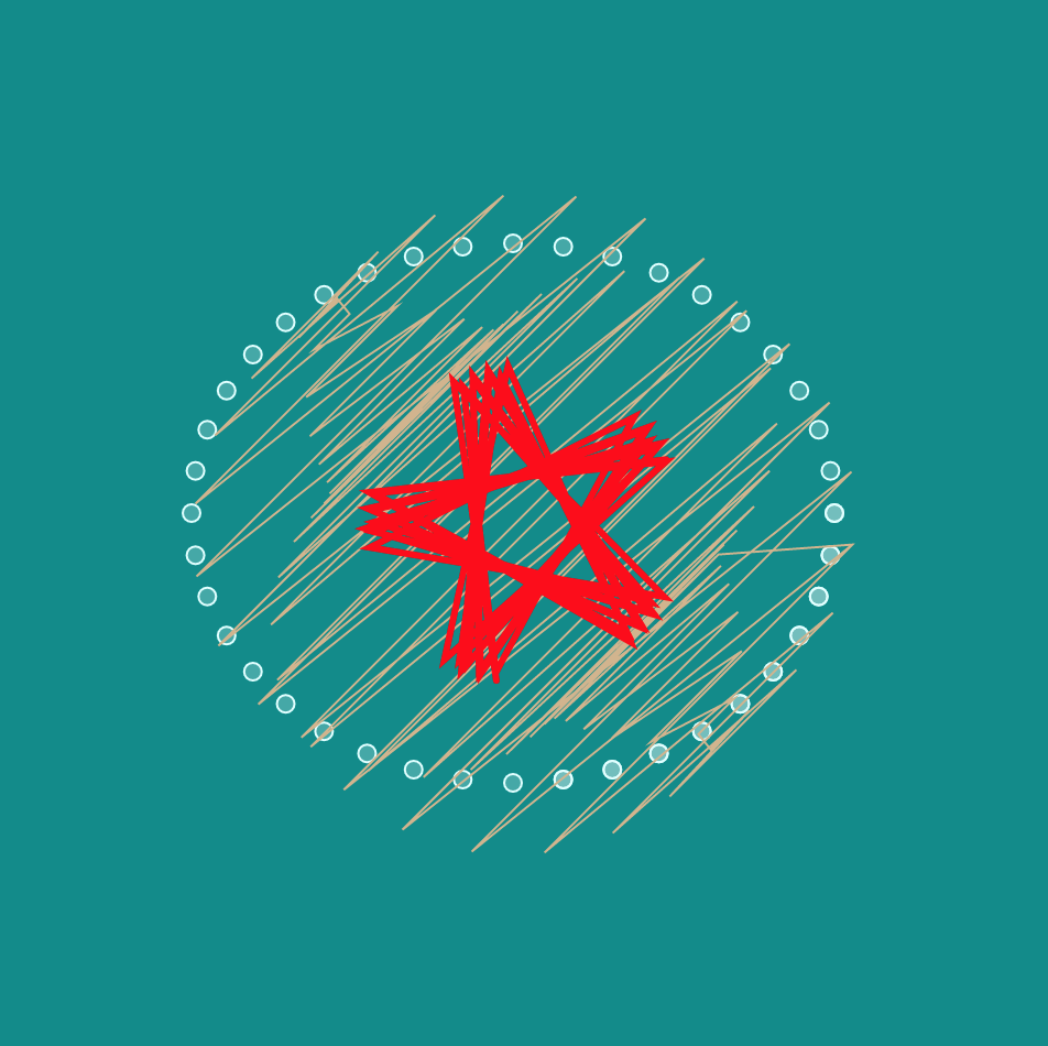
//Project - 07 - Curves
var nPoints = 100;
function setup() {
createCanvas(400, 400);
}
function draw() {
fill(20, 8, 78); //color for background
rect(0, 0, width, height);
push();
translate(width / 1.4, height / 2);
drawCurve();
pop();
}
function drawCurve() {
var cR = map(mouseX, 0, width, 100, 200);
var cG = map(mouseX, 0, width, 200, 250);
var cB = map(mouseX, 0, width, 230, 255); //color for shape
var s = 100; // size
var a = constrain(mouseX/2, 0, width) / 30; // mousex position
var b = constrain(mouseY/2, 0, height) / 30; // mousey position
fill(cR, cB, cG);
strokeWeight(5);
stroke(255);
beginShape();
for (var i = 0; i < nPoints; i++){
var t = map(i, 0, nPoints, 0, TWO_PI);
x = s * (cos(a+t) * (1-(cos(a+t))));
y = s * (sin(b+t) * (1-(cos(b+t)))); // equation of curve to create shape
vertex(x,y);// drawing vertex
}
endShape(CLOSE);
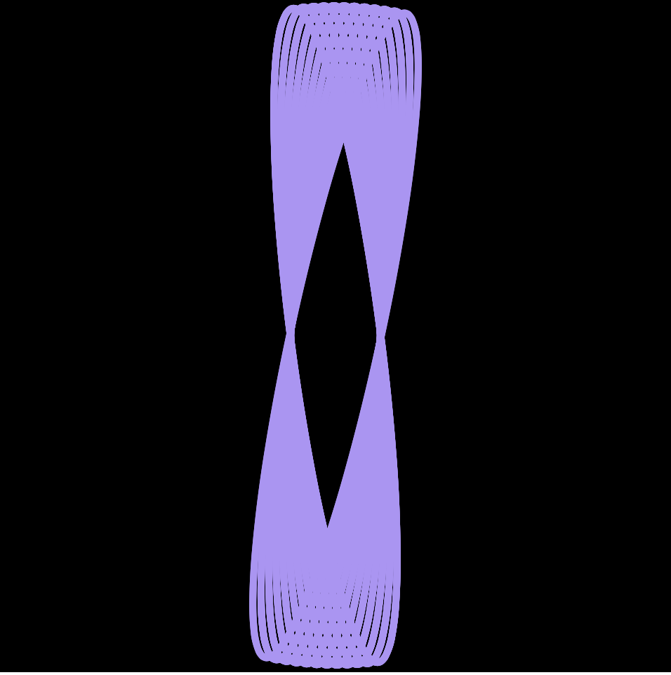
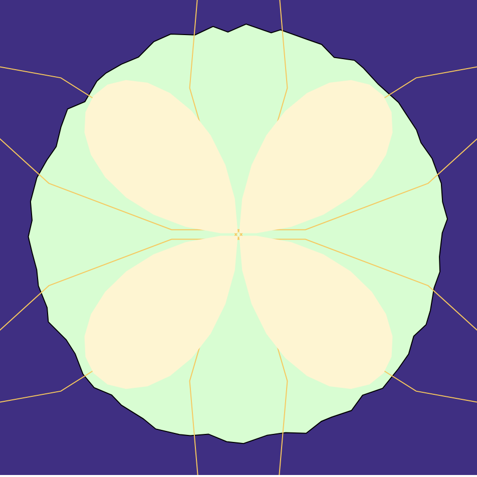
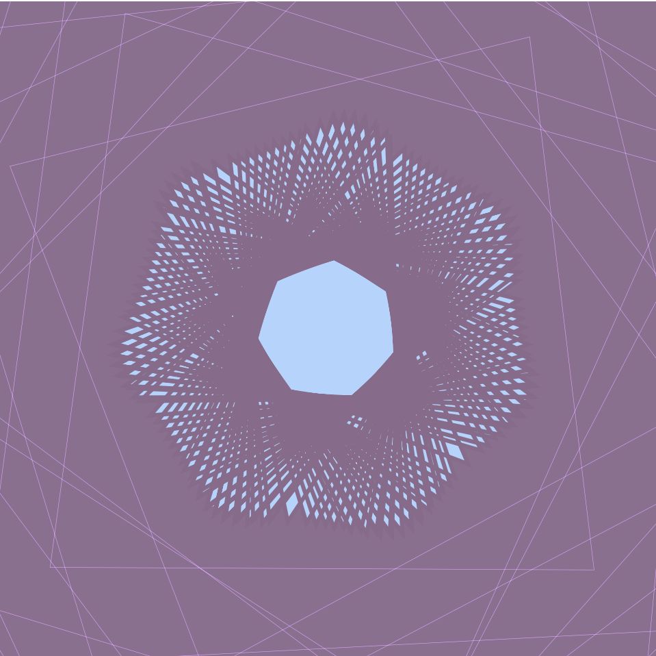
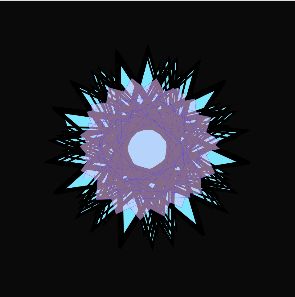
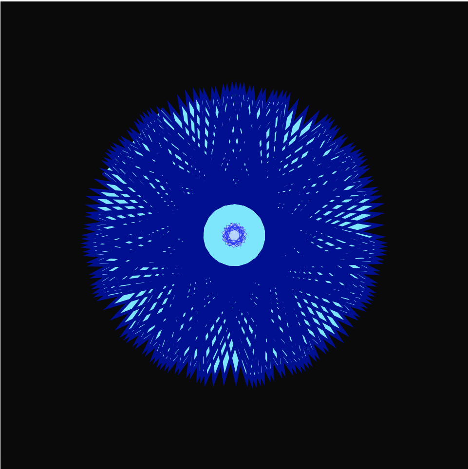
}I used the Cardioid Curve from the Mathworld curves site to create this project. At first, I thought the movement of the curve was interesting, which is why I chose to use this particular curve. I thought the circular movement of the curve looked like the tornado-like movement of water when it is spun. I tried to express that circular movement of water with cardioid. By making the background color dark blue and the shape itself change colors between different shades of blue, I tried to express water and the spiral movement of water. Everytime I move the mouse left, the shape will turn clockwise and the color will turn vivid blue-green. When the mouse is moved right, the shape will turn counter-clockwise and the color will turn light blue.