Month: October 2018

Curves

// Jessica Timczyk
// Section D
// jtimczyk@andrew.cmu.edu
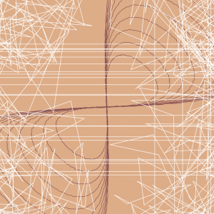
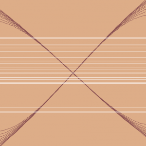
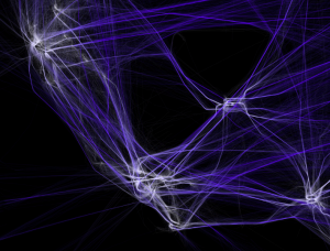
// Project-07-Curves

// Global Variables
var z;
var colorR;
var colorG;
var colorB;


function setup() {
    createCanvas(480, 480);
    z = -width / 4;
}

function draw() {
    background(255, 215, 250);
    translate(width / 2, height / 2, z);
    rotate(map(mouseX, 0, width, 0, TWO_PI)); // allow curve to rotate
    colorR = map(mouseY, 0, height, 0, 100); // variables for color transition
    colorG = map(mouseY, 0, height, 70, 100);
    colorB = map(mouseY, 0, height, 100, 220);
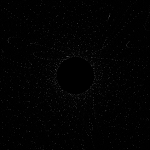
    drawLoxodrome(0.4, map(mouseX, 0, 400, 0, 480)); // draw curves and change size as mouse moves
}

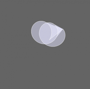
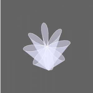
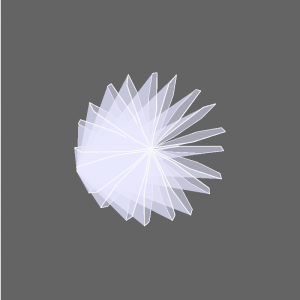
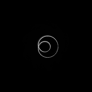
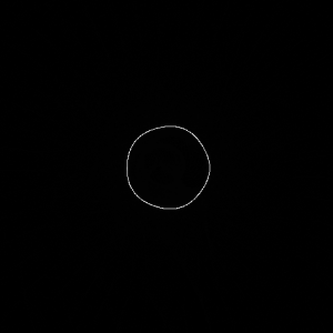
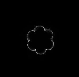
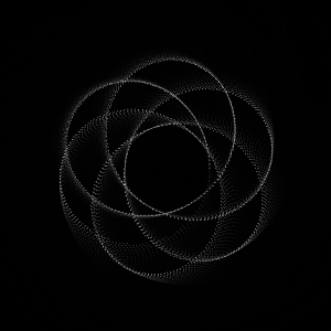
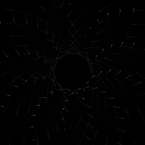
function drawLoxodrome(b, scal) { // equations for drawing the curves of the loxodrome
    for (var a = 0.4; a < 4; a += 0.2) {
        noStroke();
        fill(colorR, colorG, colorB); // fill of the curves change
        beginShape(QUAD_STRIP); // establish the begining of the curve shape
        var w = 0.1 / sqrt(a + 1);
        for (var t = -20; t < 20; t += 0.1) {
            var q = 4 + a * a * exp(2 * b * t);
            vertex(scal * 4 * a * exp( b * t) * cos(t) / q, scal * 4 * a * exp( b * t) * sin(t) / q);
            var c = a + w;
            q = 4 + c * c * exp(2 * b * t);
            vertex(scal * 4 * c * exp(b * t) * cos(t) / q, scal * 4 * c * exp(b * t) * sin(t) / q);
        }
        endShape();
    }
}

I really enjoyed doing this project, it allowed me to experiment with a bunch of different curves and shapes. Although it took a while to decide what shape to do and as well figure out the different equations and what each one does, the ending results are very interesting and intricate curves. I liked being able to manipulate and explore what each of the different parameters control. After messing with the different variables and trying to change different ones with the movements of the mouse, I  decided on having the mouse movement control the scale of the shape rather than one of the other parameters so that it would keep the main structure of the curve intact as it moved. Overall, I really enjoyed this project because it allowed me to explore more things and aspects of the code than other previous projects have allowed us.

sketch

// Han Yu
// Section D
// hyu1@andrew.cmu.edu
// Project 07

var nPoints = 200;

function setup() {
    createCanvas(400, 400, WEBGL); // create a 3D canvas
    frameRate(100);
}

function draw() {
    background(100);   
    fill(250); 
    rotateZ(millis() / 8000);
    stroke(250);    
    drawFlower();
}

function drawFlower() {
    // http://mathworld.wolfram.com/Slinky.html   
    var x;
    var y;
    var z;
    // variables inside the formula
    var p = constrain((mouseX / width), 0.0, 400);
    var q = constrain((mouseY / height), 0.0, 400.0);
    
    fill(200, 200, 255, 100.5);
    beginShape();
    stroke(250);
    for (var i = 0; i < nPoints; i++) {
        var t = map(i, 0, nPoints, 0, TWO_PI);
        
        // Flower(slinky):
        x = (PI+100*cos(10*q*t))*cos(t);
        y = (PI+100*cos(10*q*t))*sin(t);
        z = 1/2*p*t + 100*sin(10*p*t);    

        vertex(x, y, z);
    }
    endShape(CLOSE);
}

I used a slinky curve for my project. A slinky curve is a space curve which consists of a spiral wound around a helix. I altered it in order to show the formation of a flower. Overall I found this project is helpful with familiar with 3D plane and curves. Below are some screenshots of different stages of my project.