Month: October 2019

sketch

//Kristine Kim
//Section D
//younsook@andrew.cmu.edu
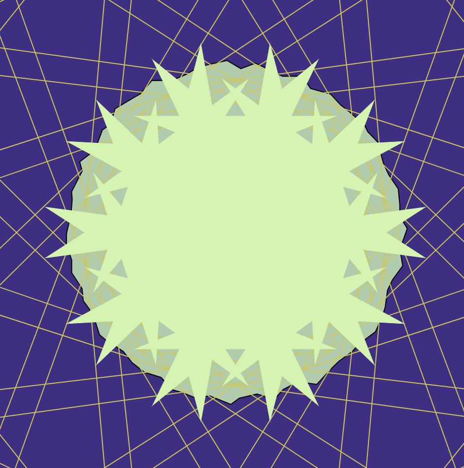
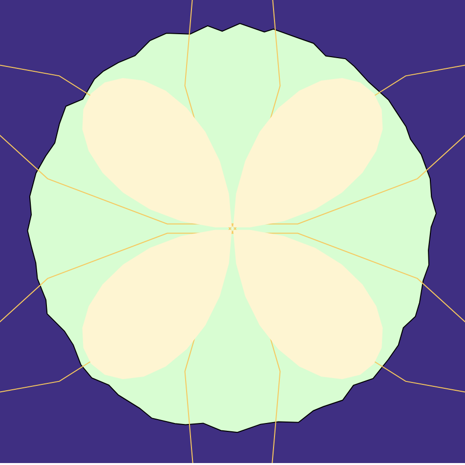
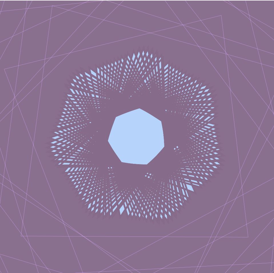
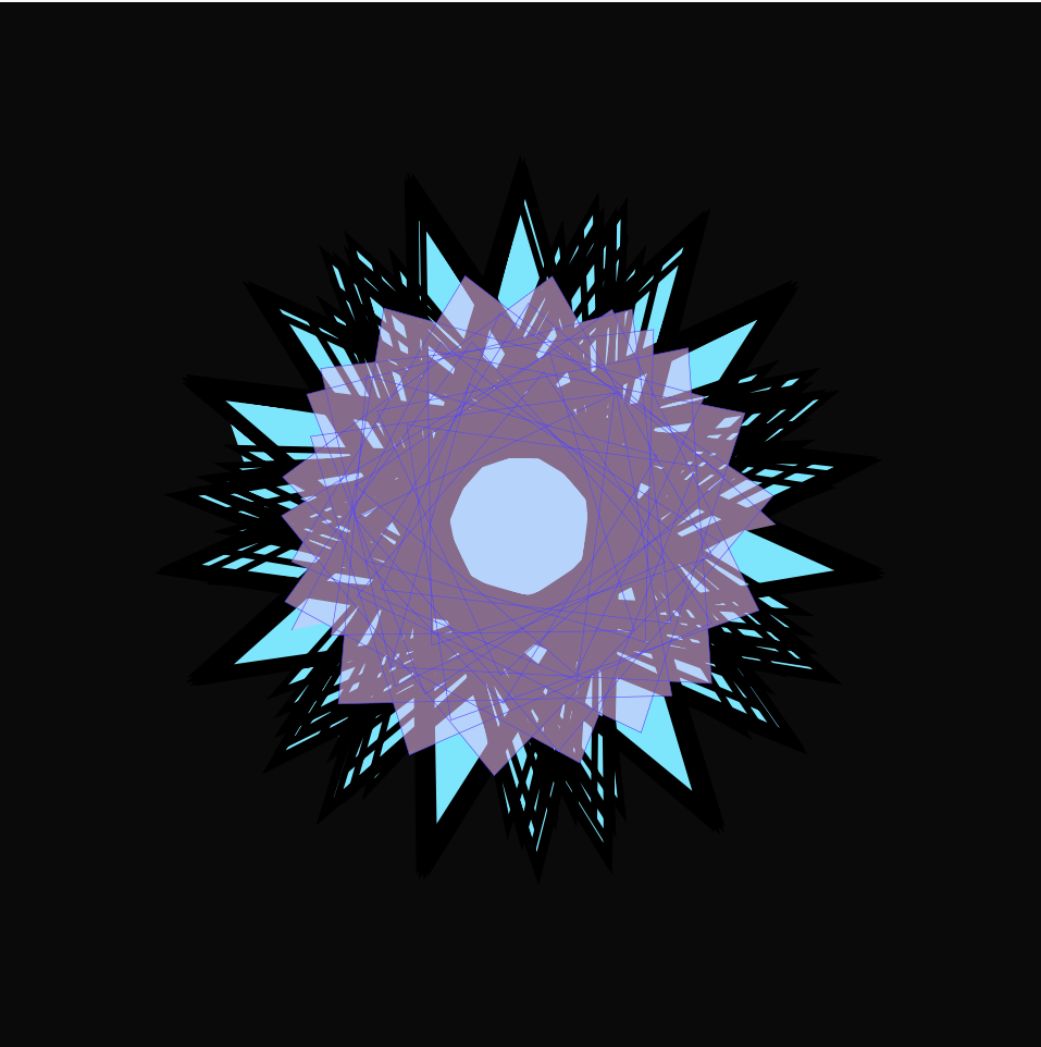
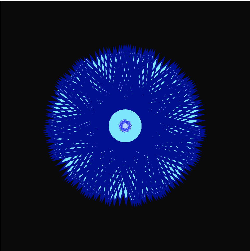
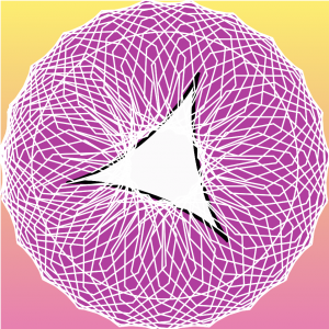
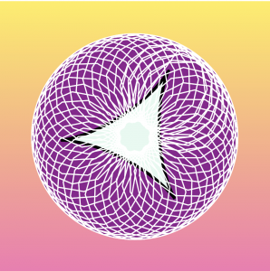
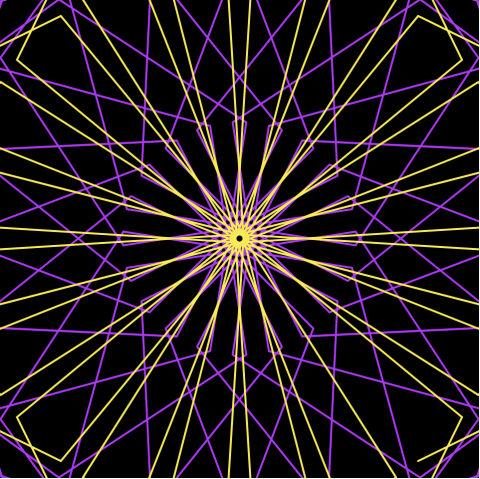
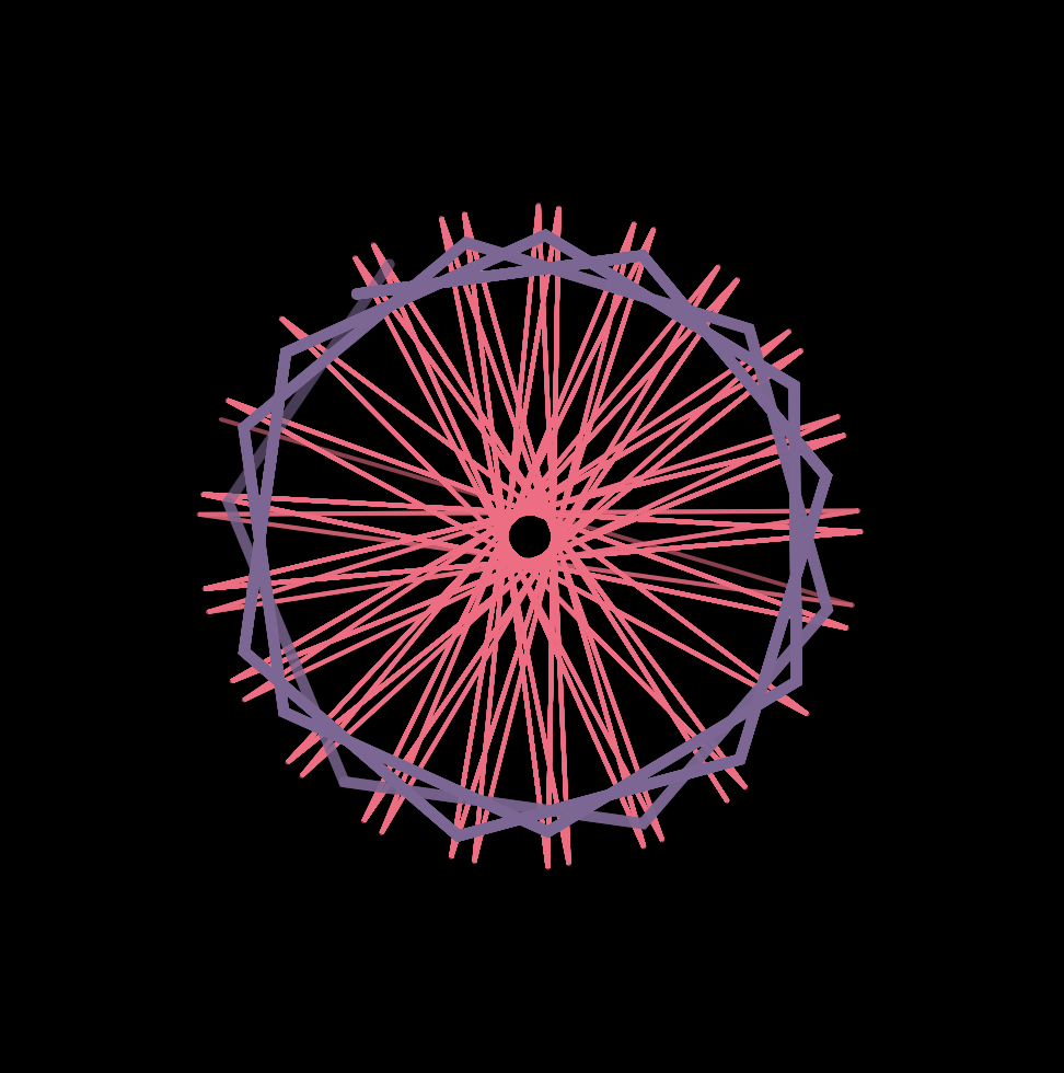
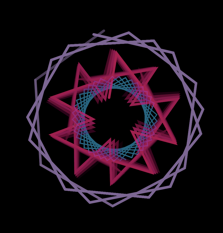
//Project- 07- Curves
var nPoints = 70

function setup() {
    createCanvas(480, 480);
    frameRate(10);
}

function draw() {
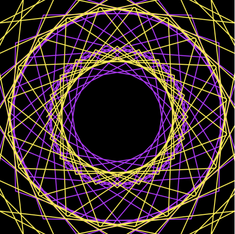
    background(67, 42, 135);
    //calling all the functions 
    //drawing all of them on the center of the canvas

    push();
    translate(width/2, height/2);
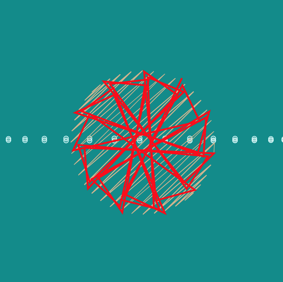
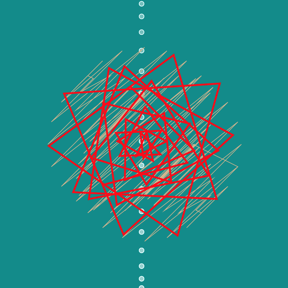
    drawMovinglines();
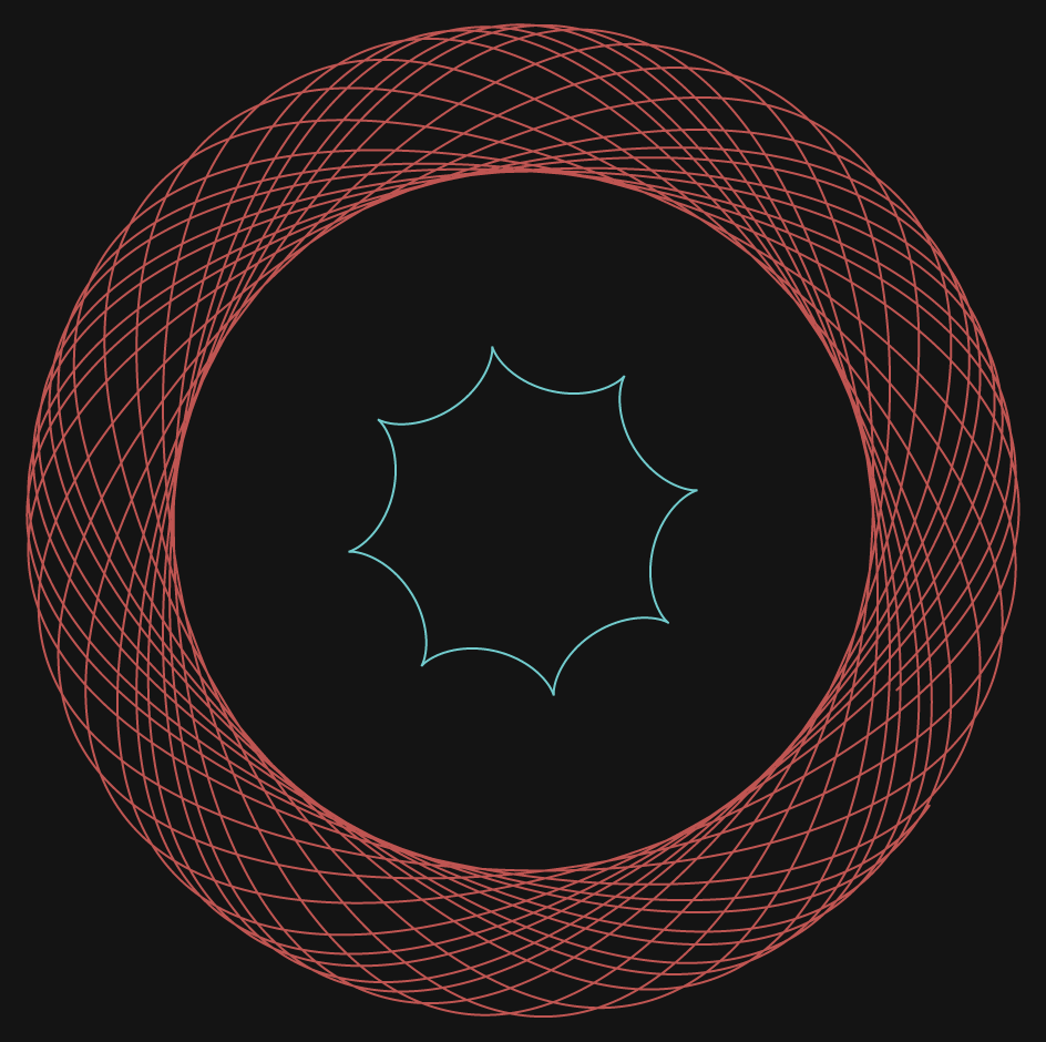
    drawHypotrochoid();
    drawEpitrochoidCurve();   
    pop();
}

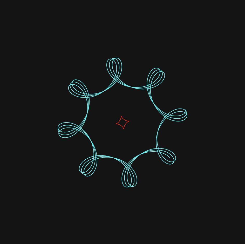
/*drawing the EpitrochoidCurve filled with
colors that are determined by mouseX and mouseY */
//the image that is drawing on top of everything
function drawEpitrochoidCurve(){

    var x;
    var y;

    var r1 = 100
    var r2 = r1 / mouseX;
    var h = constrain(mouseX, r1 , r2) 
    noStroke();
    fill(mouseY, 245, mouseX);
    beginShape();
    //for loop to draw the epitrochoidcurve
    for (var i = 0; i < nPoints; i++){
        var t = map(i, 0, nPoints, 0, TWO_PI);
        x = (r1 + r2) * cos(t) - h * cos(t * (r1 + r2) / r2);
        y = (r1 + r2) * sin(t) - h * sin(t * (r1 + r2) / r2);
        vertex (x,y);
    }
    endShape(CLOSE);
}
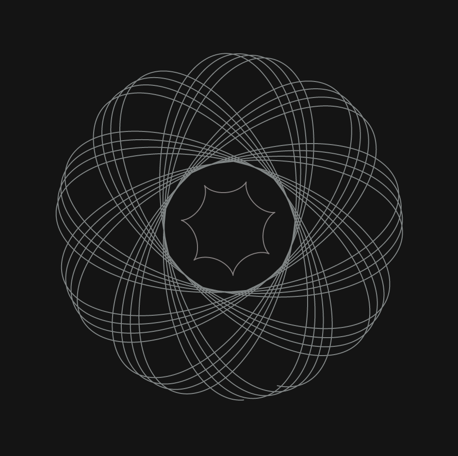
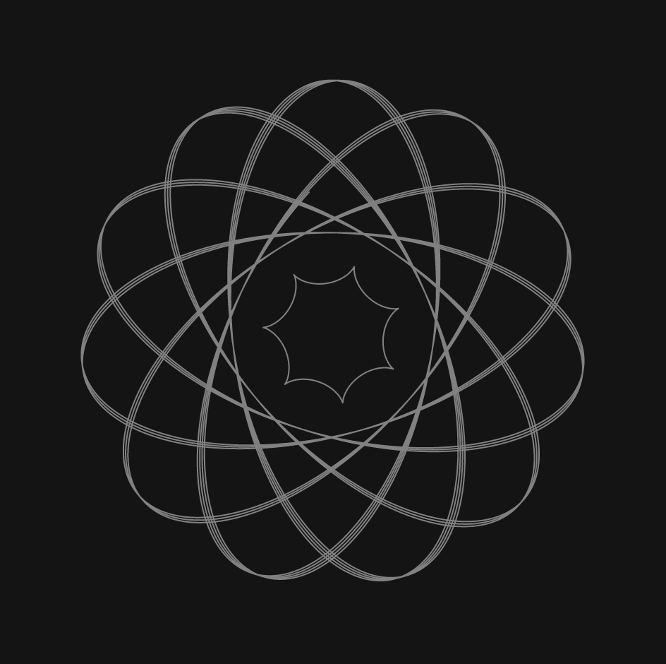
/*drawing the hypotrochoid with vertexs with
colors determined by mouseY */
//the first layer, drawing behind the epitrochoidcurve and movinglines

function drawHypotrochoid(){
    var x;
    var y;

    var r1 = 250
    var r2 = r1/ mouseX;
    var h = constrain(mouseY, r1, r2)
    stroke(mouseY, 200, 73);
    noFill();
    beginShape();
    //for loop for drawing the hypotrochoid form
    for (var i = 0; i < nPoints; i ++){
        var t = map(i, 0, nPoints, 0 , TWO_PI);
        x = (r1- r2) * cos(t) + h * cos(t * (r1 - r2) / r2);
        y = (r1- r2) * sin(t) + h * sin(t * (r1 - r2) / r2);
        vertex(x,y)
    }
    endShape(CLOSE);
}
/*drawing the constiently moving/wiggling circle
the radius and fill all controlled by mouseX and mouseY
the second layer, between the epitrochoidcurve and hypotrochoid */

function drawMovinglines(){
    var x;
    var y;
    var r1 = mouseX
    fill(mouseX, mouseY, mouseX)

    beginShape();
    //for loop for drawing the wiggling circle
    for (var i = 0; i < nPoints; i++) {
        var t = map(i, 0, nPoints, 0, TWO_PI);
        var x = r1 * cos(t);
        var y = r1 * sin(t);
        vertex(x + random(-5, 5), y + random(-5, 5));
    }
    endShape(CLOSE);

}
    

I was first very intimidated by this project because it looked so complicated and intricate, but I studying the website provided to us was very helpful. The little explanations and gif helped me understand the concept a lot. There are just so many ways we can execute this project so I struggled with starting the project, but once I drew the Hypotrochoid function, I knew how to approach this project. I played around with the quantity of nPoints, fill(), stroke(), and a lot with mouseX and mouseY until I ended up with the product that I have right now . I enjoyed creating this a lot because I love discovering new images and findings so I was pleasantly surprised every single time I changed something in my code and found different drawings.

sketch

//Lauren Park
//ljpark@andrew.cmu.edu
//Section D
//Project-07-Curves

function setup() {
  createCanvas(480, 480);
}

function draw() {
  background(10);
  
  drawHypotrochoid();
  drawHypocycloid();
}

function drawHypotrochoid() {
  var x;
  var y;
  
  //mouse controls color change for stroke
  var r = constrain(mouseX, 0, 300);
  var g = constrain(mouseY, 0, 300);
  var b = 150;
  
  push();
  fill('#53E9FF');
  stroke(r, g, b);
  strokeWeight(3);
  translate(width/2, height/2);
  
  //control hypotrochoid
  var ha1 = map(r, 0, width, 0, 100);
  var ha2 = map(g, 0, height, 0, 100);
  
  beginShape();
  for (var i = 0; i < 480; i+=3) {
    var angle1 = map(i, 0, 250, 0, 360);
  
  //equation of hypotrochoid from MathWorld curves site
  x = (ha1 - ha2)* cos(angle1) + b * cos((ha1 - ha2 * angle1));
  y = (ha1 - ha2)* sin(angle1) - b * sin((ha1 - ha2 * angle1));
  vertex(x, y);
  }
  endShape();
  pop();
}

function drawHypocycloid() {
  var x;
  var y;
  
  //mouse controls color change for stroke
  var r = map(mouseX, 0, width, 50, 255);
  var g = map(mouseY, 0, height, 50, 255);
  
  push();
  fill(254, 193, 255, 140);
  stroke(r, g, 255);
  strokeWeight(0.3);
  translate(width/2, height/2);
  
  //control hypocycloid
  var hy1 = map(mouseX, 0, width, 0, 300);
  var hy2 = map(mouseY, 0, height, 0, 300);
  
  beginShape();
  for (var a = 0; a < 200; a+=3) {
    var angle2 = map(a, 0, 100, 0, 360);
    
    //equation of hypocycloid from MathWorld curves site
    x = (hy1 + hy2)* cos(angle2) + hy2* cos((hy1 + hy2)*angle2);
    y = (hy1 + hy2)* sin(angle2) - hy2* sin((hy1 + hy2)*angle2);
    vertex(x, y);
  }
  endShape();
  pop();
}

My idea for this project initially came from visuals of a rotating flower. However, throughout this process of figuring out this project, I became more interested in intricate patterns within this flower shape. And so, I was more focused on adding different color changes and perspectives when the mouse moves, to show off different designs of this form. When the mouse is somewhere near the top left edge of the canvas, I want to show the two different curves separately to represent seed-like forms, so that when the mouse moves in other directions, then the flower can gradually grow and spread to a wider view. Overall, it was very challenging but very satisfying to create patterns that remind of the kaleidoscope effect.

sketch

//Monica Chang
//mjchang@andrew.cmu.edu
//Section D
//Project-07-Curves

var nPoints = 100;
var radiusX;
var radiusY;
var separation = 125;

function setup() {
    createCanvas(480, 480);
  
}

function draw() {
    background("darkcyan");
    fill(255, 255, 255, 64);
    
    radiusX = mouseX;
    radiusY = mouseY;

    drawCircles();
    drawEpitrochoidCurve();
    drawDeltoid();
}

//circle elements

function drawCircles() {
  
  // a sequence of little, circle elements
    push();
    translate(width / 2, height / 2);
    for (var i = 0; i < nPoints + 10; i++) {
        var theta = map(i, 0, nPoints, 0, TWO_PI);
        var px = radiusX / 2 * cos(theta);
        var py = radiusY / 2 * sin(theta);
      
        stroke("lightcyan");
        strokeWeight(1);
        circle(px - 5, py - 5, 8, 8);
    }
    pop();
  
}


function drawDeltoid() {
    //Deltoid:
    //http://mathworld.wolfram.com/Deltoid.html
    beginShape();
    nPoints = 40;
    for (var i = 0; i < nPoints; i++) {   
    	var angle = map(i, 0, 180, 0, 360);
        var radius = 70;
        var a = map(mouseX, 0, height, 5, 80)
        var b = map(mouseY, 0, height, 5, 90)
        
        //x-coordinate for deltoid
        var x = (a - b) * cos(angle) + radius * cos((a - b * angle));
        //y-coordinate for deltoid
        var y = (a - b) * sin(angle) - radius * sin((a - b * angle));
        rotate(radians(angle));
        noFill();
        strokeWeight(3);
        stroke("red");
        vertex(x, y);
      }
    endShape();
    

}

function drawEpitrochoidCurve() {
    // Epicycloid:
    // http://mathworld.wolfram.com/Epicycloid.html
    
    var x2;
    var y2;
    
    var a = 80.0;
    var b = a / 2.0;
    var h = constrain(mouseY / 8.0, 0, b);
    var ph = mouseX / 30.0;
    
    noFill();
    stroke("tan");
    strokeWeight(1);
    beginShape();
    translate(width / 2, height / 2);
    for (var i = 0; i < nPoints + 10; i++) {
        var t = map(i, 0, nPoints, 0, TWO_PI);
        
        x2 = (a + b) * cos(t) - h * cos(ph + t * (a + b) / b);
        y2 = (a + b) * sin(t) - h * sin(ph + t * (a + b) / b);
      
        //switching x and y-coordinates to create a band of waves/
        vertex(x2, y2);
        vertex(y2, x2);
    }
    endShape(CLOSE);
    
}

This project definitely had me studying the formulas 75% of the time for me to really start putting anything together. However, once I got the gist of the formulas, it was really entertaining for me. I began with studying the deltoid curve and I realized this particular curve created so many different shapes. Thus, I wanted to provide a more constant curve which became the sequence of circles which are relatively more static to create a sense of balance.