Month: October 2021

My Project

//cbtruong;
//Section B;

//sets up the variables for stroke color;
//col is the stroke color for smooth conical spiral;
//col2 is the stroke color for the rough conical spiral;
var col = 0;
var col2 = 0;
//sets up the variable for angl to allow for rotation;
var angl = 0;
//sets up the variable for the shifting fill color value;
//for the rough conical spiral;
var shiftingVal = 100;
//sets up the variable that allows for reversing the change;
//of shiftingVal;
var shiftingValChange = 1;


function setup() {
    createCanvas(480, 480);
    background(220);
    text("p5.js vers 0.9.0 test.", 10, 15);
}

function draw() {
    background(220);
    stroke(0);
    //diagonal lines that hit the center of the spirals;
    line(0, 0, 120, 120);
    line(0, 480, 120, 360);
    line(480, 0, 360, 120);
    line(480, 480, 360, 360);
    //lines that outline the perimeter of the canvas;
    line(0, 0, 480, 0);
    line(0, 0, 0, 480);
    line(480, 0, 480, 480);
    line(0, 480, 480, 480);
    //lines of the innerbox whose vertices are the spiral centers;
    line(120, 120, 120, 360);
    line(120, 360, 360, 360);
    line(360, 360, 360, 120);
    line(360, 120, 120, 120);

    //draws the middle, rough concial spiral;
    strokeWeight(2);
    fill(shiftingVal);
    stroke(col2);
    push();
    translate(240, 240);
    conicalSpiralTopViewRough();
    pop();
    
    //draws the 4 smooth rotating conical spirals;
    noFill();
    stroke(col);
    for (var i = 120; i <= 360; i += 240){
        for (var j = 120; j <= 360; j += 240){
            push();
            translate(j, i);
            rotate(radians(angl));
            scale(0.5);
            conicalSpiralTopViewSmooth();
            pop();
        }
    }

    //checks if the shiftingVal is too high or low;
    //if too high, the fill becomes darker;
    //if too low, the fill becomes ligher;
    if (shiftingVal >= 255){
        shiftingValChange = shiftingValChange * -1;
    }
    else if (shiftingVal < 100){
        shiftingValChange = shiftingValChange * -1;
    }
    //changes the shiftingVal;
    shiftingVal += 1*shiftingValChange;
    //changes the angle and allows for rotation;
    //of the smooth conical spirals;
    angl += 0.1;
    

}

//function that creates the smooth conical spirals;
function conicalSpiralTopViewSmooth() {
    //variables for h, height; a, angle; r, radius;
    var h = 1;
    var a;
    var r = 30;
    
    //adds interactivity;
    //as one goes right, the size of the spiral increases;
    //as one goes down, the complexity of the spiral increases;
    var indepChangeX = map(mouseX, 0, 480, 500, 1000);
    var indepChangeY = map(mouseY, 0, 480, 800, 1000);
    a = indepChangeY;

    //actually creates the spiral;
    beginShape();
    for (var i = 0; i < indepChangeX; i++){
        var z = map(i, 0, 400, 0, PI);
        x = ((h - z) / h)*r*cos(radians(a*z));
        y = ((h - z) / h)*r*sin(radians(a*z));
        vertex(x, y);
    }
    endShape(CLOSE);

}

//function that creates the rough middle conical spiral;
function conicalSpiralTopViewRough() {
    //variables are the same as the smoothSpiral function;
    var h = 0.5;
    var a = 1000;
    var r;
    
    //adds interactivity;
    //the radius is now dependant on mouseY, going up increases size;
    //going left increases complexity;
    r = map(mouseY, 0, 480, 20, 10);
    var edgeNum = map(mouseX, 0, 480, 60, 30);
    
    //creates the spiral;
    beginShape();
    for (var i = 0; i < edgeNum; i++){
        var z = map(i, 0, 50, 0, TWO_PI);
        x = ((h - z) / h)*r*cos(radians(a*z));
        y = ((h - z) / h)*r*sin(radians(a*z));
        vertex(x, y);
    }
    endShape();
}

//mousePressed function that changes the variables col and col2;
//with random values of r, g, and b;
function mousePressed() {
    var randR = random(150);
    var randG = random(150);
    var randB = random(150);
    col = color(randR, randG, randB);
    col2 = color(randR + random(-50, 50), randG + random(-50, 50), randB + random(-50, 50));
}

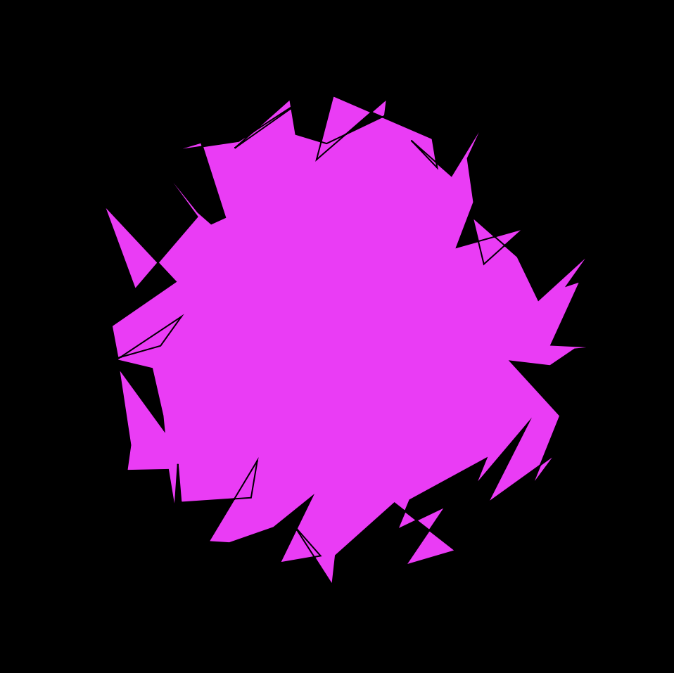
I initially had no idea what to make in terms of curves. That was until I happened upon the Conical Spiral. It was supposed to be 3-D, but it ended up as a top down view of a spiral which I liked. Overall, I liked what I did with this Project.

As for how it works, clicking the mouse will change the colors of the middle “rough” Conical Spiral and the 4 “smooth” Conical Spirals. The colors of both types are similar but not the same, as seen with the use of random() in the code.

Along with that, moving the mouse right will increase the size of the “smooth” Spirals and reduce the size and complexity of the “rough” Spiral. Moving left does the opposite. Moving down increases the complexity of the “smooth” Spirals while also reducing the size of them and the “rough” Spiral.