![[OLD FALL 2019] 15-104 • Introduction to Computing for Creative Practice](../../../../wp-content/uploads/2020/08/stop-banner.png)
// lee chu
// section c
// lrchu@andrew.cmu.edu
// project - 07
// variables for equation
var angle;
var t;
var x;
var y;
var xx;
var yy;
// characteristics of shapes
var sizes = [];
var size;
var ct;
var step;
// color
var r;
var g;
var b;
function setup() {
createCanvas(480, 300);
noFill();
strokeWeight(0);
angle = 0;
t = 20;
// create sizing for layers
for (h = 0; h < 60; h ++) {
sizes.push(h * 3);
}
size = 20;
ct = 200;
// color control
r = 36;
g = 33;
b = 40;
step = 5;
}
function draw() {
background(r, g, b);
// change turn direction and rate
if (mouseX < width / 2 & mouseX > 0 && mouseY < height && mouseY > 0) {
angle -= (width / 2 - constrain(mouseX, 0, width / 2)) / width / 2 / 6;
}
if (mouseX > width / 2 & mouseX < width && mouseY < height && mouseY > 0) {
angle += (constrain(mouseX, width/2, width) - width / 2) / width / 2 / 6;
}
// generate shapes
for (j = 0; j < sizes.length; j ++) {
cata(sizes[sizes.length - j]);
r = (r + step * (j + 1)) % 255;
g = (g + step * (j + 1)) % 255;
b = (b + step * (j + 1)) % 255;
}
deltoid(sizes[1]);
}
function cata(size) {
fill(r, g, b);
push();
translate(width / 2, height / 2);
beginShape();
for (i = 0; i < ct; i ++) {
t = map(i, 0, ct, 0, 2 * PI);
xx = 3 * cos(t) + cos(3 * t + 2 * angle) - cos(2 * angle);
yy = - 3 * sin(t) + sin(3 * t + 2 * angle) - sin(2 * angle);
vertex(xx * size, yy * size);
}
endShape();
pop();
}
function deltoid(sizeD) {
fill('black');
push();
translate(width / 2, height / 2);
beginShape();
for (i = 0; i < ct; i ++) {
t = map(i, 0, ct, 0, 2 * PI);
x = 2 * cos(t) + cos(2 * t);
y = -2 * sin(t) + sin(2 * t);
vertex(x * sizeD, y * sizeD);
}
endShape();
pop();
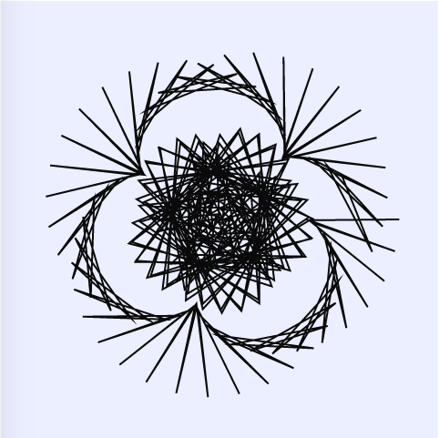
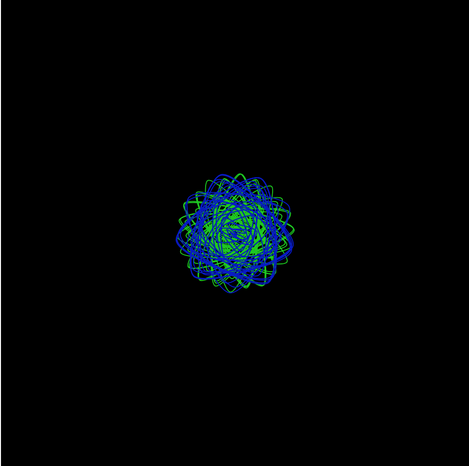
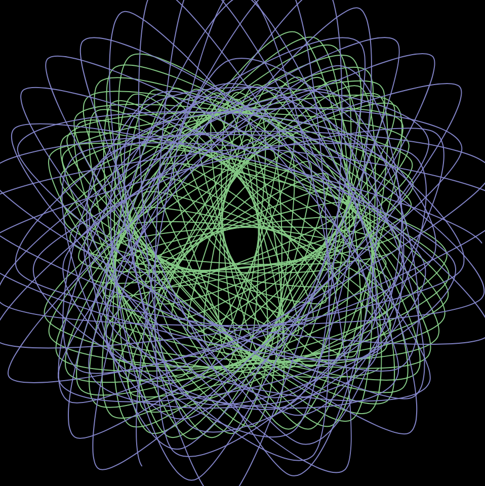
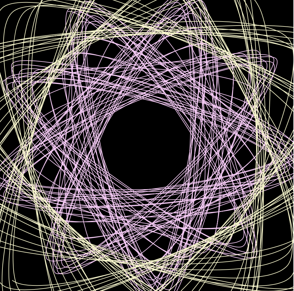
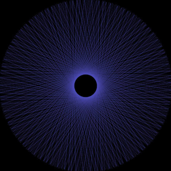
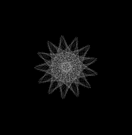
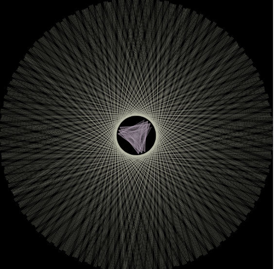
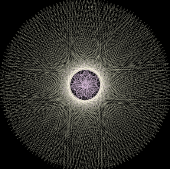
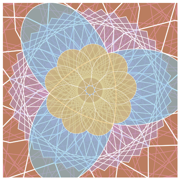
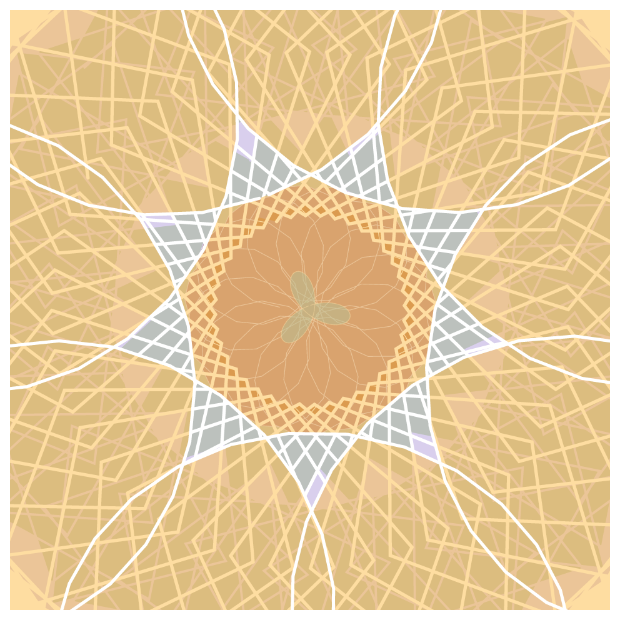
}I was intrigued by the deltoid catacaustic, which consists of the deltoid, a triangle bowing in, and the catacaustic which circumscribes the deltoid as it rotates around its axis. The center of all the layers of the catacaustic is the black deltoid in the middle of the canvas.