![[OLD FALL 2019] 15-104 • Introduction to Computing for Creative Practice](../../../../wp-content/uploads/2020/08/stop-banner.png)
//Jamie Park           jiminp@andrew.cmu.edu
//15-104          Section E        Project 7

//Global Variables
var maxIVal = 300;

function setup(){
    createCanvas(450, 450);
    frameRate(40);
}

function draw(){
    background("black");
    drawHypotrochoid();
    drawRanunculoid();
    drawHypotrochoid2();
    drawAstroid();
}

function drawRanunculoid(){
        //http://mathworld.wolfram.com/Ranunculoid.html

    //push and translate the drawing to the center of the canvas
    push();
    translate(width / 2, height / 2);

    //constrain mouseX and map mouse movement
    var canvaWidth = constrain(mouseX, 0, width);
    var angle = map(canvaWidth, 0, width, 0, 360);
    var a = map(canvaWidth, 0, width, 10, width / 18);

    //change stroke color according to mouse movement, begin shape, and rotate
    noFill();
    stroke(canvaWidth, 150, canvaWidth - 20);
    beginShape();
    rotate(radians(angle));

    //forLoop that creates the shape
    for (var i = 0; i < TWO_PI; i += 0.1){
    //equation for the shape and vertex (high points)
        var x = a * (6 * cos (i) - cos (6 * i));
        var y = a * (6 * sin (i) - sin (6 * i));
        vertex(x, y);
    }
    endShape();
    pop();
}

function drawHypotrochoid(){
    //http://mathworld.wolfram.com/Hypocycloid.html

    //push and translate the drawing to the center of the canvas
    push();
    translate(width / 2, height / 2);

    //constrain mouseX, mouseY and map mouse movement
    var canvaLength = constrain(mouseX, 0, width);
    var canvaHeight = constrain(mouseY, 0, height);
    var a = map(canvaLength, 0, width, 10, width / 30);
    var b = map(canvaHeight, 0, height, 2, height / 30);
    var radAngle = 200;

    //change stroke color according to mouse movement and begin shape
    noFill();
    stroke(230, canvaHeight, canvaLength);
    beginShape();

    //forLoop that creates the shape
    for (var i = 0; i < maxIVal; i++){
        //variable rotation that maps the i value into angles
        var rotation = map(i, 0, 360, 0, 360);
        //equation for the shape and vertex
        var x = (a - b) * cos(rotation) + radAngle * cos((a - b * rotation));
        var y = (a - b) * sin(rotation) - radAngle * sin((a - b * rotation));
        vertex(x, y);
    }
    endShape();
    pop();
}

function drawHypotrochoid2(){
    //http://mathworld.wolfram.com/Hypocycloid.html

    //push and translate the drawing to the center of the canvas
    push();
    translate(width / 2, height / 2);

    //constrain mouseX, mouseY and map mouse movement
    var canvaLength = constrain(mouseX, 0, width);
    var canvaHeight = constrain(mouseY, 0, height);
    var a = map(canvaLength, 0, width, 2, width / 60);
    var b = map(canvaHeight, 0, height, 2, height / 60);
    var radAngle = 100;

    //change stroke color according to mouse movement and begin shape
    noFill();
    stroke(canvaLength, canvaHeight, 10);
    beginShape();

    //forLoop that creates the shape
    for (var i = 0; i < maxIVal; i += 2){
        //variable rotation that maps the i value into angles
        var rotation = map(i, 0, 360, 0, 270);
        //equation for the shape and vertex
        var x = (a - b) * cos(rotation) + radAngle * cos((a - b * rotation));
        var y = (a - b) * sin(rotation) - radAngle * sin((a - b * rotation));
        vertex(x, y);
    }
    endShape();
    pop();
}

function drawAstroid(){
    //http://mathworld.wolfram.com/Astroid.html

    push();
    translate(width / 2, height / 2);

    //variables necessary to define the curve
    var canvaLength = constrain(mouseX, 0, width);
    var a = map(canvaLength, 0, width, 20, width * 0.25);
    var angle = map(canvaLength, 0, width, 0, 360);
    //creating the curve
    noFill();
    stroke(100, canvaLength, canvaLength);
    beginShape();
    rotate(radians(angle));

    //forLoop for the curve and the math equation for the curves
    for (var i = 0; i < (2 * PI); i += 0.1){
        var angle = map(i, 360, 0, TWO_PI);
        var x = a * pow(cos(i), 3);
        var y = a * pow(sin(i), 3);
        vertex(x, y);
    }
    endShape();
    pop();
}
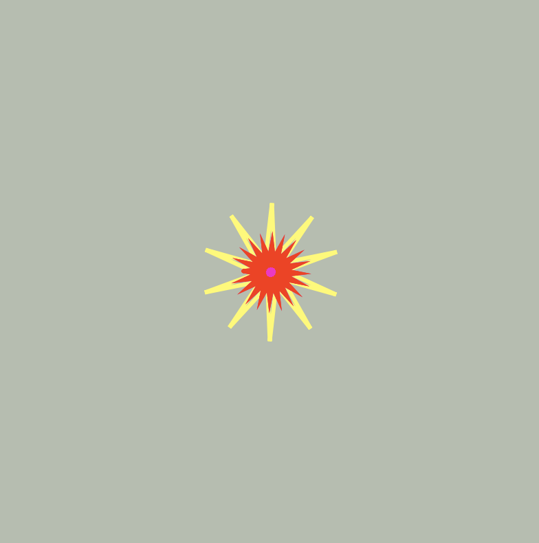
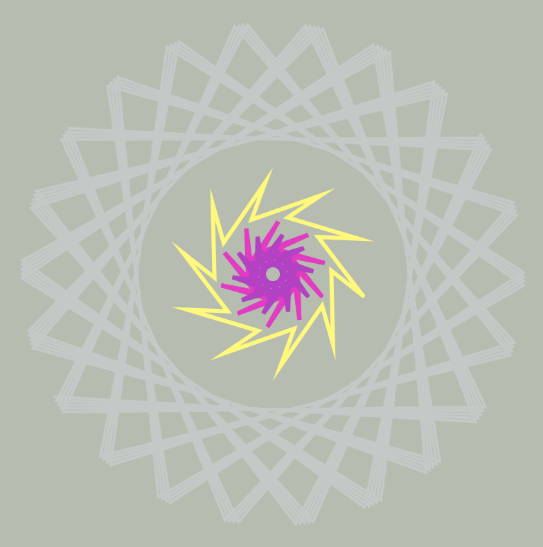
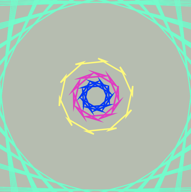
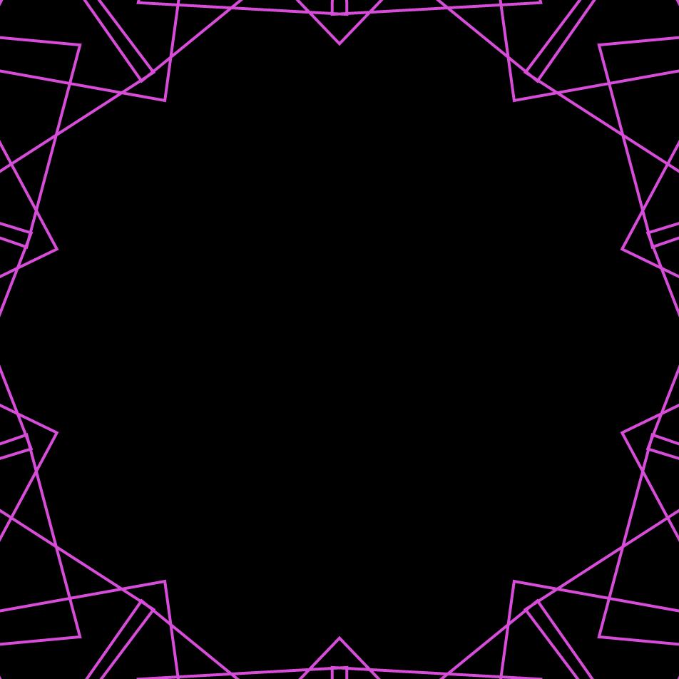
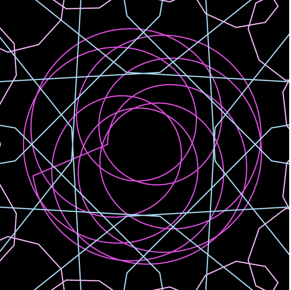
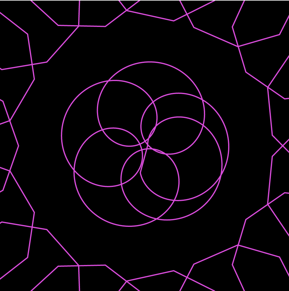
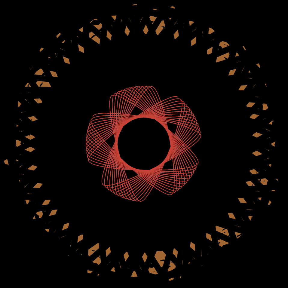
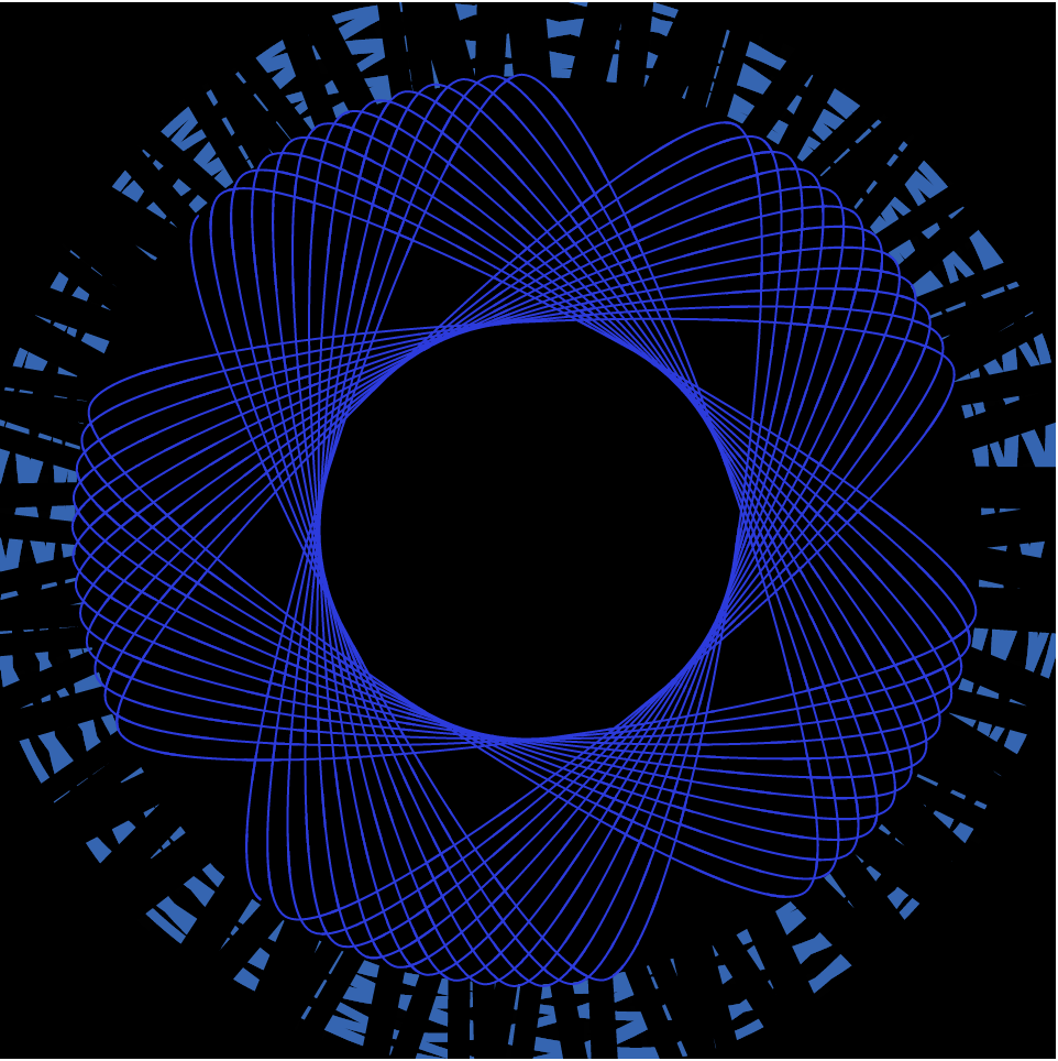
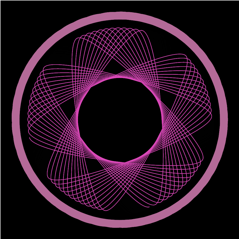
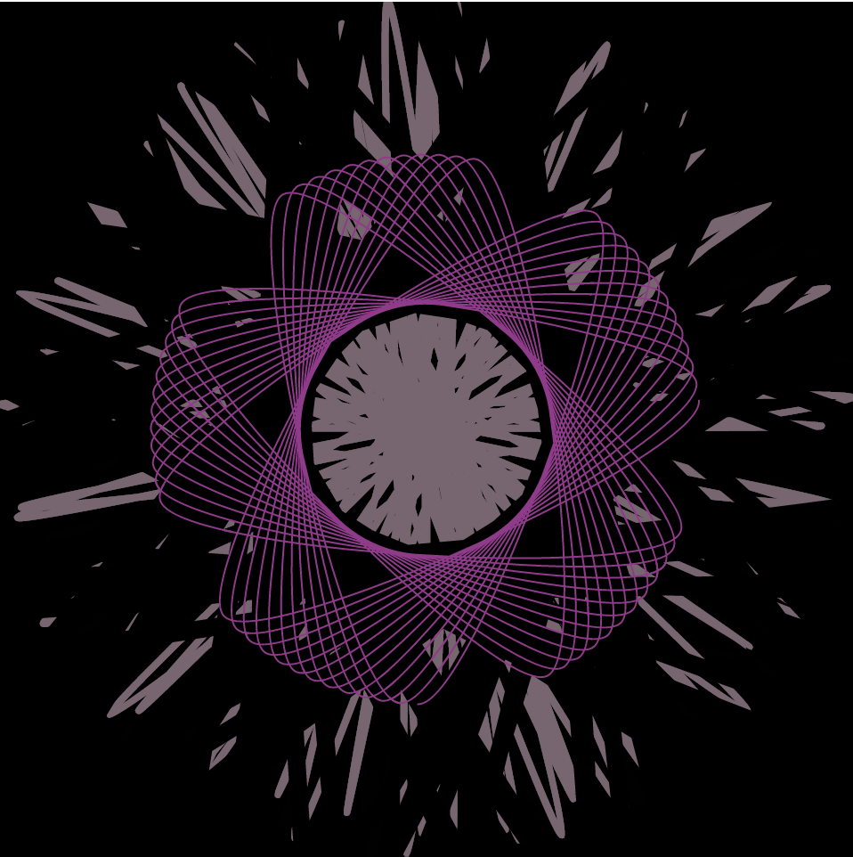
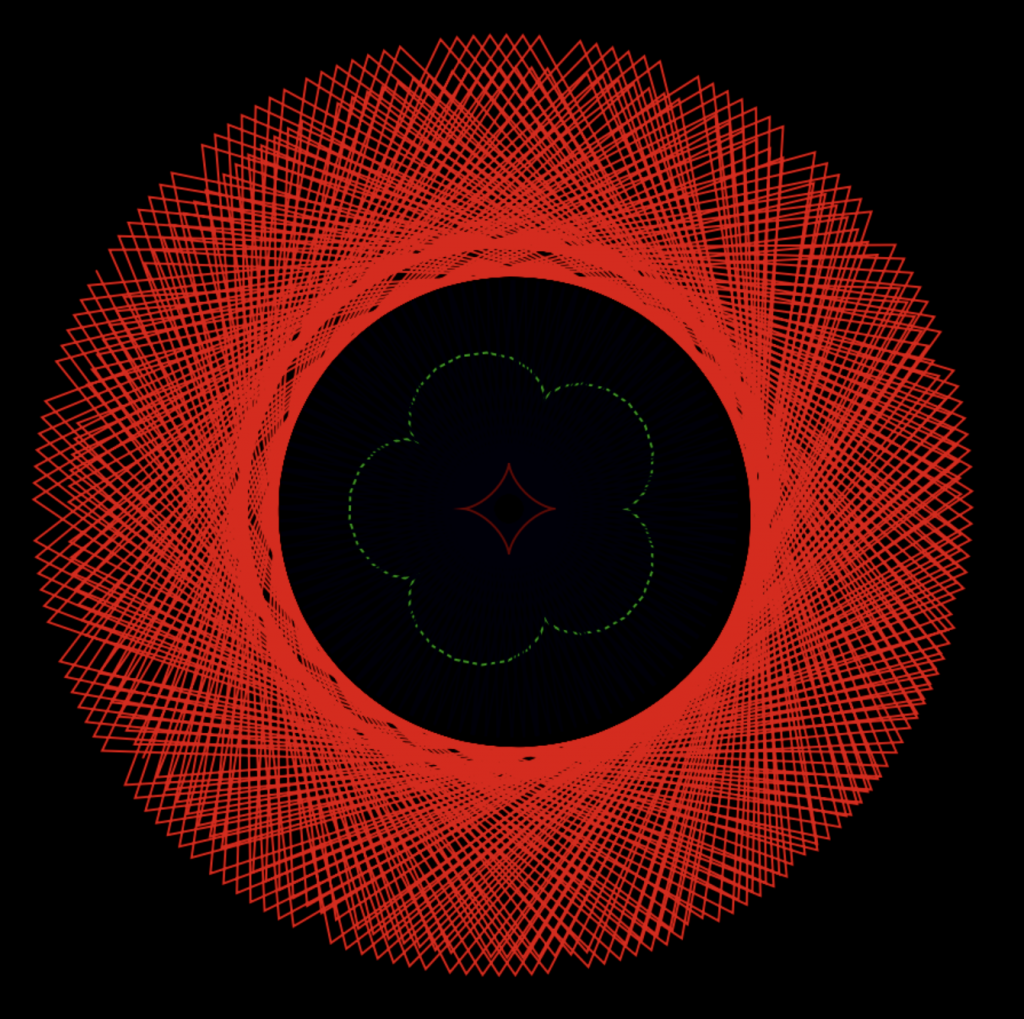
Similar to others, I struggled with understanding how to start the project. But after spending some time decoding the code on “notes” and “deliverables” sections, I had a good grasp on how things were supposed to be done. I ended up creating four curves that change color and size/complexity according to the mouse position. I am happy with the way it turned out.
Top left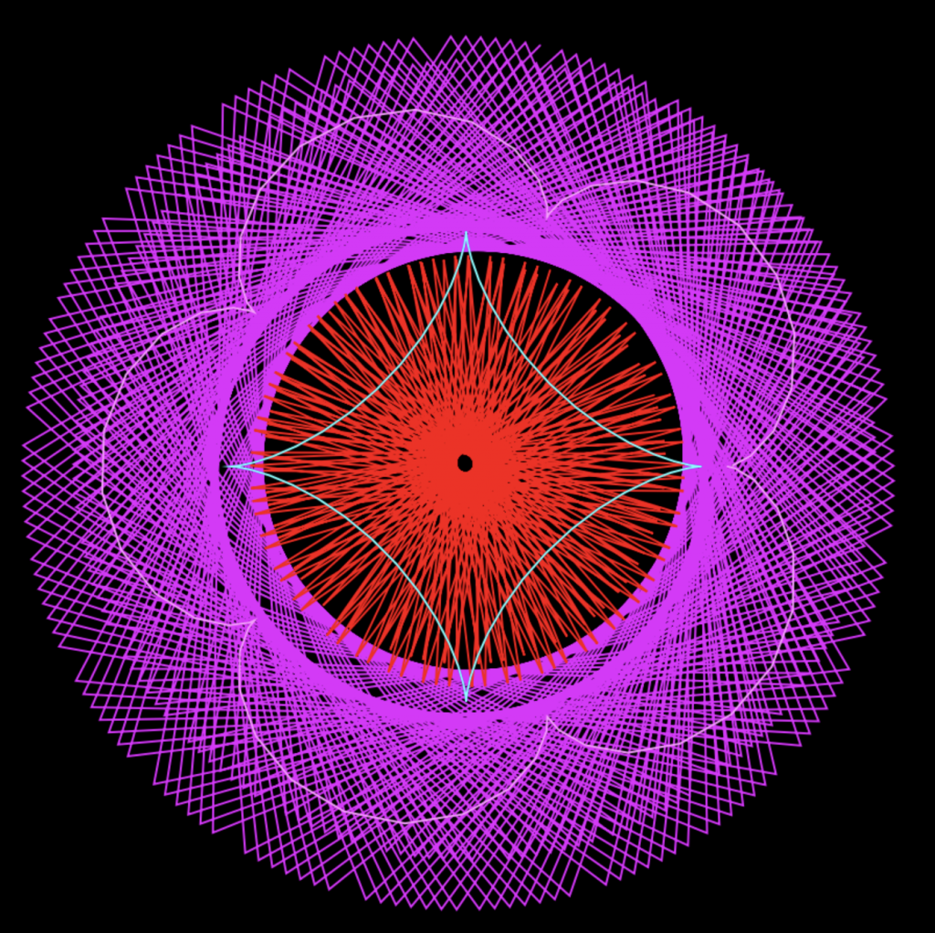
Top Right 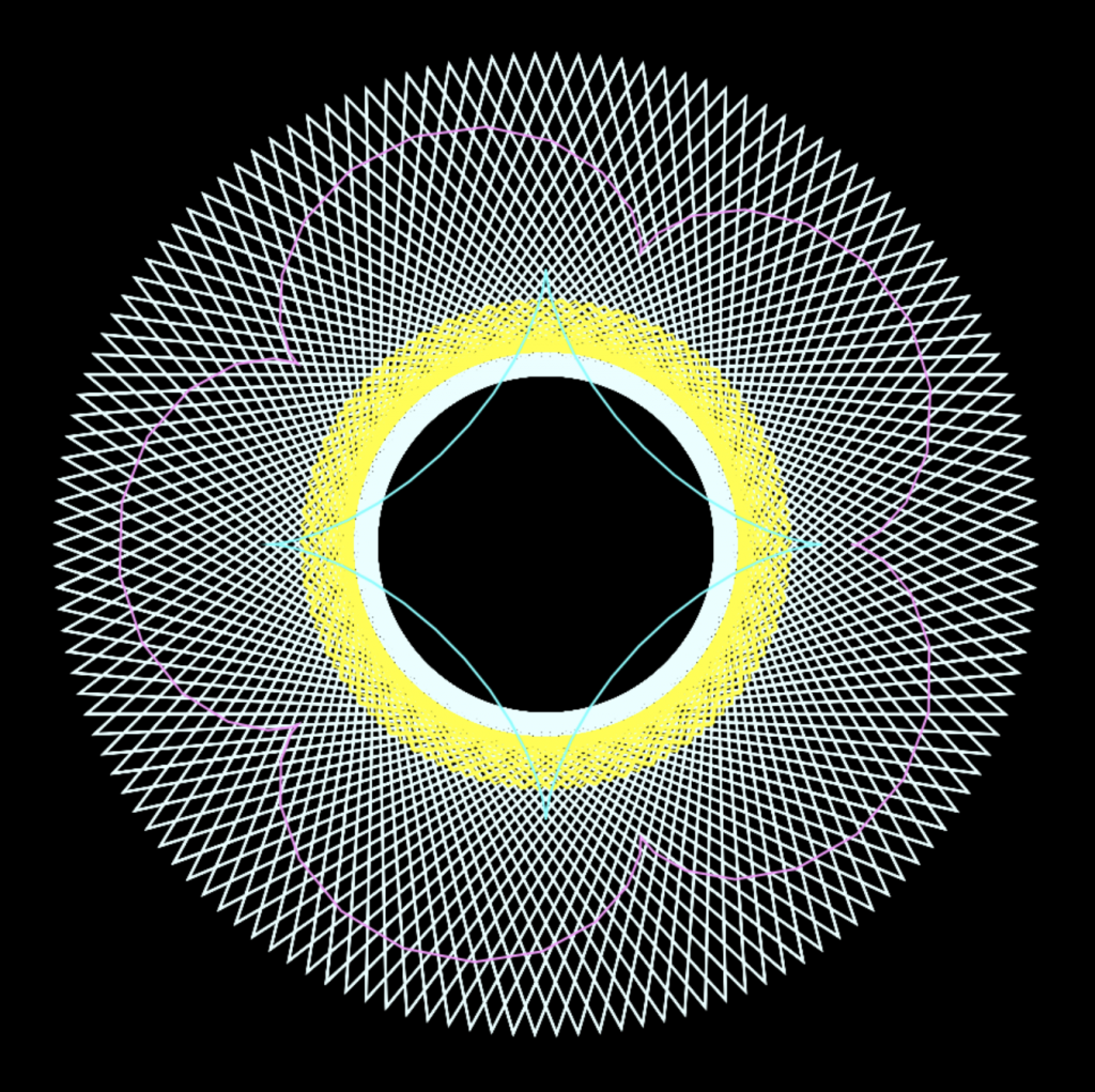
Bottom Left 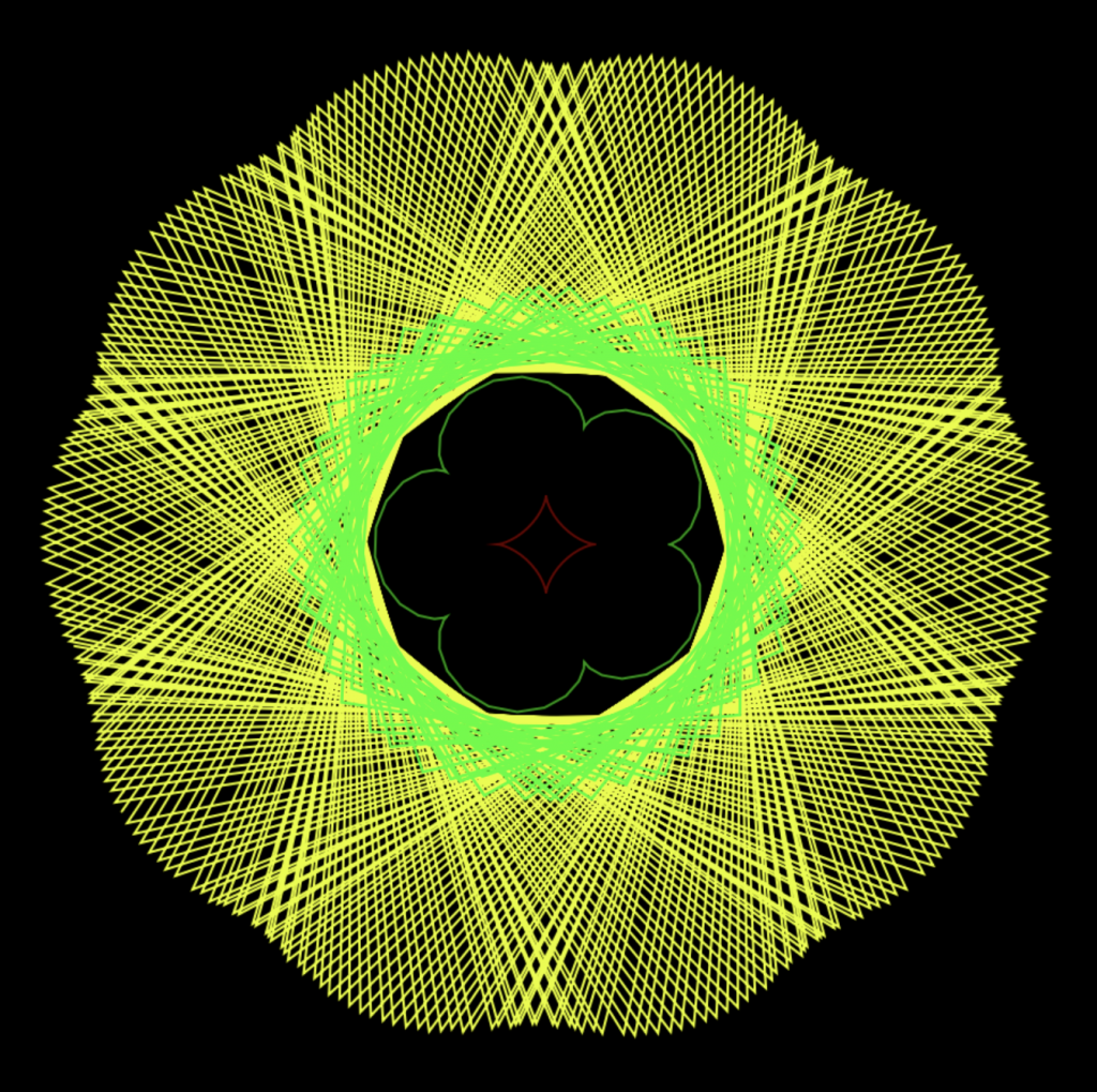
Bottom Right