sketch
//Jonathan Perez
//Section B
//jdperez@andrew.cmu.edu
//Project 7

var a = 100 // inner asteroid diagonal radius
var b = 100 // second inner asteroid diagonal radius
var a2 = 200 //outer astroid diagonal radius
var b2 = 200 //second outer astroid diagonal radius
var lineArrayX = [a, a, a, a, a, a, a, a, a, a, a, a, a, a, a, a, a]
var lineArrayY = [0, 0, 0, 0, 0, 0, 0, 0, 0, 0, 0, 0, 0, 0, 0, 0, 0]
var lineLength = 30
var lineSize = 5
function setup() {
    createCanvas(480, 480);
    background(255);
}

function draw() {
    background(255);
    mouseDistX = dist(mouseX, height/2, width/2, height/2); //X distance from center
    mouseDistY = dist(width/2, mouseY, width/2, height/2); //Y distance from center
    a = map(mouseDistX, 0, 240, 0, 150) //maps X distance from center to max a value
    b = map(mouseDistY, 0, 240, 0, 150); //maps Y distance from center to max b value
    a2 = map(mouseDistX, 0, 240, 0, 300); //maps X distance from center to max a2 value
    b2 = map(mouseDistY, 0, 240, 0, 300); //maps Y distance from center to max b2 value
    traceAstroid(height/2, width/2, a, b);
    drawAstroid(height/2, width/2, a2, b2);
}


//drawing line asteroid
function traceAstroid(x, y, a, b) {
    asteroidX =  a * pow(cos(millis()/1000), 3);// x parametric for an astroid x = acos^3(t)
    asteroidY =  b * pow(sin(millis()/1000), 3);// y parametric for an asteroid y = asin^3(t)
    push();
    translate(x, y);
    for(i = 0; i < lineArrayX.length; i++) {
        fill(255 - i*255/lineArrayX.length); //fades line into background
        noStroke();
        if(i < lineArrayX.length - 1){ //if not the leading point
            //trails behind the leading point
            lineArrayX[i] = lineArrayX[i+1]
            lineArrayY[i] = lineArrayY[i+1]
        } else { //if the leading point
             //next X and Y coordinates
            lineArrayX[i] = asteroidX
            lineArrayY[i] = asteroidY
        }
        ellipse(lineArrayX[i], lineArrayY[i], lineSize, lineSize);
        ellipse(-lineArrayX[i], -lineArrayY[i], lineSize, lineSize);
    }
    pop();
}


//outer asteroid
function drawAstroid(x, y, a2, b2) {
    push();
    translate(width/2, height/2);
    rotate(TWO_PI/8); //eighth rotation so that inner astroid touches the inside walls
    for(i = 0; i < 472; i++) { // 472 stops the astroid exactly halfway down the vertical sides
        asteroidX2 = a2 * pow(cos(i/200), 3); // x parametric for an astroid x = acos^3(t)
        asteroidY2 = b2 * pow(sin(i/200), 3); // y parametric for an asteroid y = asin^3(t)
        fill(0);
        noStroke();
        ellipse(asteroidX2, asteroidY2, lineSize, lineSize);
        ellipse(-asteroidX2, -asteroidY2, lineSize, lineSize);

    }
    pop();
}
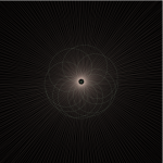
I thought this project was super fun… I haven’t had the chance to do any sort of geometry or math in a while, and this was a nice way to sort of flex those old muscles.
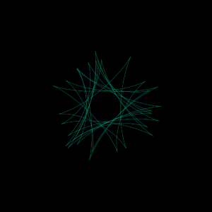
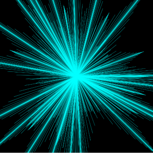
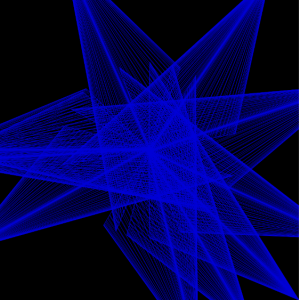
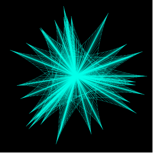
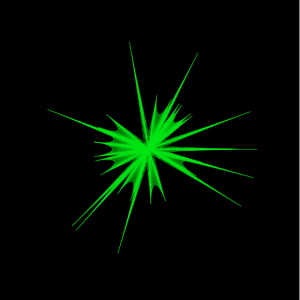
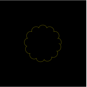
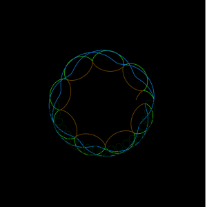
To start off, I just clicked around on the geometry site provided for us. I was just looking for a curve that both looked feasible to implement (with out smoke coming out of my ears) and aesthetically interesting. Eventually I stumbled across the astroid, and decided, sure, let’s use that.
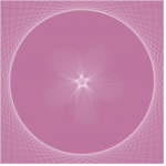
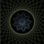
After that, I just started playing around with how I could draw the shape and modify it. I knew right off the bat that I wanted to do something with a trailing point… so that was actually the first part I coded. After that I added the second rotated astroid (to make the whole image an astroid evolute).
On their own, these shapes aren’t super exciting. Originally, since the astroid is a hypocycloid, I was going to play around with the number of points in the curve (instead of just four points). Instead, I went a rotation direction instead. Well, I say rotation, but nothing is truly rotating in the image. In the code, the distance between diagonal points is being altered, to create the illusion of rotation. I thought that was pretty cool, especially with the trailing point moving around. To me this animation feels like a card turning around on one point.
![[OLD FALL 2017] 15-104 • Introduction to Computing for Creative Practice](../../../../wp-content/uploads/2020/08/stop-banner.png)
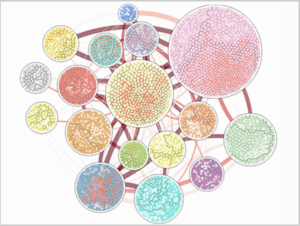
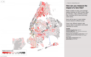
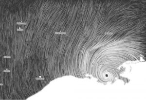
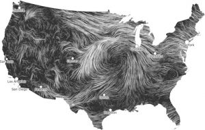
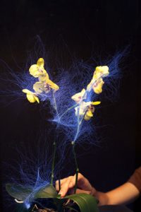
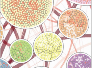 (Above are pictures of the Vorograph of Cody Dunne, Michael Muller, Nicola Perra, Mauro Martino, 2015)